DhruvaKumar Model Predictive Control Save
MPC in vehicle to track reference trajectory
Model predictive controller

This project was done as a part of Udacity's Self-Driving Car Engineer Nanodegree Program. It implements a Model Predictive Controller (MPC) to control a car in order to follow a reference trajectory as closely as possible. The state of the car and the reference trajectory waypoints are provided by Udacity's simulator. At every time step, the MPC provides the actuator inputs (steering angle and throttle) back to the simulator that minimizes a cost function. The communication is through uWebSockets.
Dependencies
- cmake >= 3.5
- make >= 4.1(mac, linux), 3.81(Windows)
- gcc/g++ >= 5.4
-
uWebSockets
- Run either
install-mac.shorinstall-ubuntu.sh
- Run either
- Ipopt and CppAD: Please refer to this document for installation instructions.
- Eigen. This is already part of the repo so you shouldn't have to worry about it.
- Simulator. You can download these from the releases tab.
- Not a dependency but read the DATA.md for a description of the data sent back from the simulator.
Basic Build Instructions
- Make a build directory:
mkdir build && cd build - Compile:
cmake .. && make - Run it:
./mpc.
Implementation
Model
The MPC uses a simple kinematic bicycle model:
x[t] = x[t-1] + v[t-1]*cos(psi[t-1])*dt
y[t] = y[t-1] + v[t-1]*sin(psi[t-1])*dt
psi[t] = psi[t-1] + v[t-1]/Lf*delta[t-1]*dt
v[t] = v[t-1] + a[t-1]*dt

cte[t] = y[t-1] - f(x[t-1]) + v[t-1]*sin(epsi[t-1])*dt
epsi[t] = psi[t-1] - psides[t-1] + v[t-1]/Lf*delta[t-1]*dt
State: [x, y, psi, v, cte, epsi]
x, y, psi: vehicle's 2d pose (position, yaw)
v: velocity
cte: cross track error (distance between vehicle's position and reference trajectory)
epsi: orientation error (angle between vehicle's orientation and reference trajectory's orientation)
Actuator inputs: [delta, a]
delta: steering angle
a: acceleration/throttle
Lf is the distance between the front of the vehicle and the center of gravity
Actuator constraints:
delta: [-25, 25] // steering angle is between -25 and 25 degrees
a: [-1, 1]
Cost function:
- Squared sum of
cteandepsiacross all time steps in the predicted horizon - Squared sum of difference between
vand a reference velocity to encourage the vehicle to stay at the reference velocty in case other terms in the cost function drop to zero - Squared sum of
deltaandato minimize the use of actuators. - Squared sum of
delta[t]-delta[t-1]anda[t]-a[t-1]to minimize sequential actuator inputs for temporal smoothness.
The weights of these terms in the cost function was manually tuned.
At every time step, for the given state and reference waypoints, the objective is to find the actuator inputs that result in a predicted trajectory over a time horizon which minimizes the cost function.
Time horizon
A time horizon of T=1s with N=10 and dt=0.1 was used as suggested. Other values for N from 5-20 and dt from 0.1 to 0.3 were tried but didn't work well. More time steps N would allow the model to find potentially better actuator values than a shorter time horizon since it's looking further into the future. However, this adds in computational cost and in some scenarios, it's not worth looking so far into the future when the actual state might differ from the predicted trajectory. Lower values of dt would provide finer resolution between the predicted states and therefore the predicted trajectory. Keeping these tradeoffs in mind, the goal would be to maximize T and minimize dt.
Polymonimal fitting and preprocessing
The reference waypoints are transformed from the global coordinate system to the vehicle's coordinate system. This results in the pose being at the origin. x,y,psi=0. A 3rd degree polynomial reference trajectory is computed from the transformed waypoints.

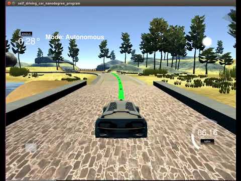
The yellow line is the reference trajectory. The green line is the predicted trajectory.
Latency
To simulate the real world latency between when an actuator command is given and when the vehicle is actuated, a 100ms latency is simulated. This is handled in the MPC by advancing the initial state of the predicted trajectory by 100 ms. The rest of the prediction follows from this delayed state.
Result