Puma Robot Simulation Save
Simulation of a Puma 762 manipulator capable of solving the Forward and Inverse Kinematics problems
Puma 762 Robot Simulation
This is a Simulation of a Puma 762 manipulator capable of solving the Forward and Inverse Kinematics problems.
The Code can also be found in Matlab File-Exchange and is based on '3D Puma Robot Demo' from Don Riley. The work provides a general analysis of the PUMA 762 kinematics and their solution methodology. There is also a description of the Graphical User Interface (GUI) used, its functions and the code developed to further enhance its capabilities and functions. Some changes were made to the functions so as to give a more complete solution for the inverse kinematics problem (position and orientation). The GUI has been enhanced with some new features. An 'Inverse Kinematics' panel for IK variables input, Radiobuttons for viewing different solutions, a 'D-H parameters' table and a 'Transformation matrix' table. The 'Demo' button has been changed to 'Draw' with some new 'drawings' available.
The PUMA 762 Manipulator
The PUMA 762 Robotic Manipulator is one of the most widely spread robots, used in production lines, mainly in automatic welding applications, but also in many university laboratories around the world.
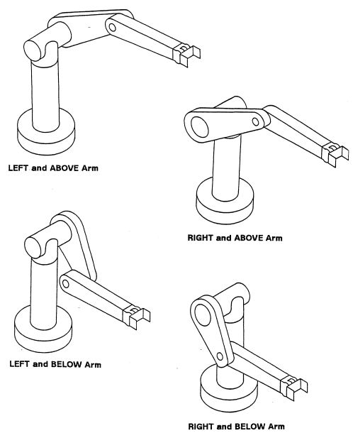
The manipulator simulates the human arm, imitating the left or right side of the human body (torso, shoulder, elbow, and wrist) according to its setup. Originally developed for General Motors, it was based on drawings by Scheinman, while at Stanford University.
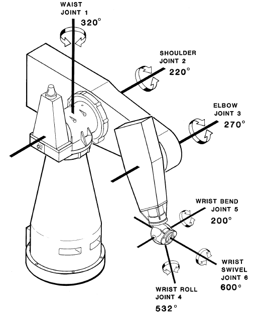
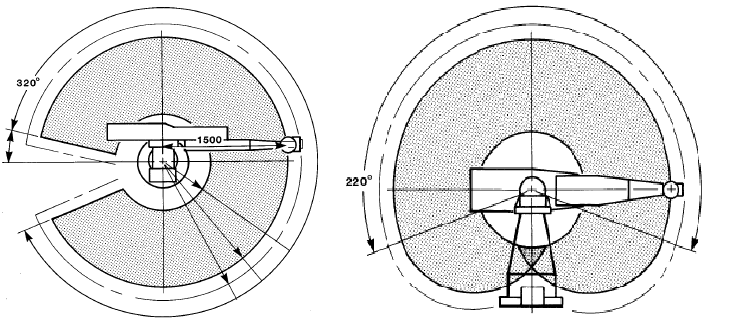
The six joints of the robot are revolute with their limitations are illustrated in Figure 1. The joints are properly positioned to give the arm six degrees of freedom. His workplace is roughly made up of a sphere with a radius of 1.25 meters (Figure 2).
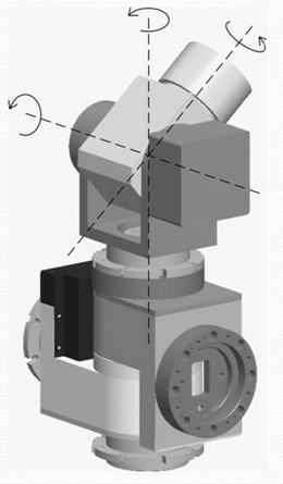
The end-effector of the arm is a Spherical wrist which means that the last three axes intersect at a common point (Figure 3). This is a sufficient condition for a six-rotary operator to have a closed-form solution. We will see the importance of this feature in the next section.
Robot Kinematics
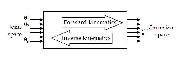
The kinematics problem in robots is divided into two separate problems. The Forward Kinematic Problem and the Inverse Kinematic Problem.
The Forward Kinematic Problem is defined as follows:
Given all the variables (angles or displacements) of the joints, we want to calculate the position and direction of the end-effector's frame relative to the base frame.
The Inverse Kinematic Problem is defined as follows:
Given the position and direction of the robots' end-effector, calculate all possible sets of joint variables (angles or displacements) with which the end-effector could reach the given position.
An illustration of the two kinematics problems is given in Figure 4
The most common method used for solving the kinematics problems is that of Denavit & Hartenberg (1955) which uses homogeneous 4x4 orthogonal transforms.
For the D-H method, an axis system is attached to each joint (i) with the zi axis pointing to the axis of rotation for revolute joints or to the axis of translation for prismatic joints. The xi, point along the common normal between zi and zi-1 and it's perpendicular to it. The yi axis is positioned to satisfy the right-hand rule.
Denavit & Hartenberg have shown that only four parameters are needed to find the displacement of the arm.
These four parameters are as follows:
- θi is the joint angle from the xi-1 axis to the xi about the zi-1 axis (using the right-hand rule)
- di is the distance from the origin of the (i−1)th coordinate frame to the intersection of the zi-1 axis with the xi-1 axis along the zi-1 axis.
- ai is the distance from the intersection of the zi-1 axis with the xi axis to the origin of the ith frame along the xi axis.
- αi is the angle from the zi-1 axis to the zi axis about the xi axis
Solving the Forward Kinematics Problem
To solve the direct kinematics problem using the Denavit & Hartenberg method we first need to place the axes on the joints of the arm, making sure that the rules mentioned above are observed. This ends up with the axes as shown in Figure 5.
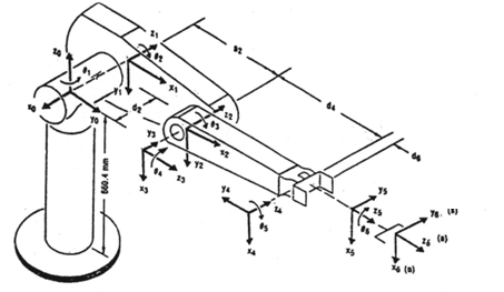
The Denavit-Hartenberg parameters of PUMA 762 are shown in Table 3.
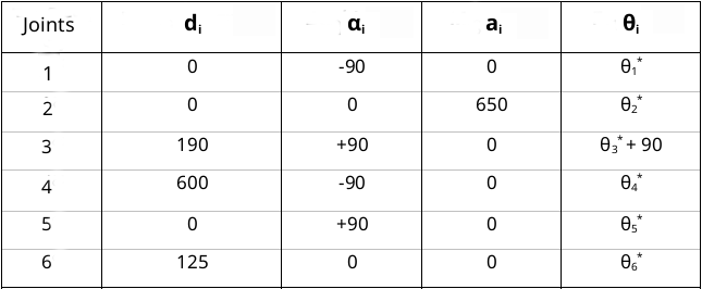
The next step requires the creation of the individual homogeneous transformations. The transformation matrices are given by the equeation (1) i-1iT = Rx (αi-1) * Dx (ai-1) * Rz (θi) * Qi (di). Where Rx, Rz denote the rotation around the x and z axes respectively, while Dx and Q denote the translation along the x and z axes respectively. The operation is as follows:
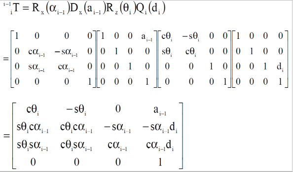
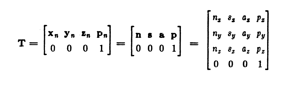
Having calculated the matrices 01T, 12T, 23T, 34T, 45T, 56T we can find the position and direction of any joint of the robot relative to the reference frame (usually the robot's base) but also to any other frame by multiplying the matrices from the reference frame to the requested link. The position of the end-effector of the arm relative to the reference frame is given by the table 06T = 01T * 12T * 23T * 34T * 45T * 56T. So the final solution is given by the table 2
In the table T (Figure 6), the elements of the last column p are the Cartesian position of the end-effector relative to the basic coordinate frame. The elements of columns 1 and 3 a and n give the normalized orientation vectors. The elements of the 2nd column s are the products of the normalized orientation vectors a and n and therefore contain no further information.
Solving the Inverse Kinematics Problem
While the Forward kinematics problem always has a unique solution, the Inverse Kinematics problem is more difficult to solve as it may have one or more solutions or none at all. The reason for this is the nonlinearity of the problem. A prerequisite for the existence of a solution is for the desired location has to be within the robot's workplace.
The solution of the inverse kinematics problem is mainly done by 2 methods, numerical and analytical (closed form) which is in turn divided into 2 sub-approaches, geometric and algebraic. In this work we used the geometric approach. This choice was made because this approach gives clear indications of which is the optimal solution for each layout of the robot, as opposed to the algebraic approach that usually requires experience by the operator and involves more calculations. The closed-form solution allows us to develop rules for choosing one particular solution among many.
Kinematic Decoupling
Solving the Inverse Problem can be simplified for arms with 6 degrees of freedom, with the last 3 links intersecting at the same point. In these cases it is possible to use kinematic decoupling, dividing the original problem into two simpler problems. These two sub-problems are called Inverse Position Kinematics and Inverse Orientation Kinematic. The first one calculates the position of the intersection of the wrist axes and the second the orientation of the wrist. This separation simplifies the calculations.
A basic requirement for the application of kinematic decoupling is that the wrist of the arm is spherical, that is to say, its three axes intersect at the same point. The arrangement of the spherical wrist whose axes z3, z4, z5 intersect at a common point is shown in Figure 7.
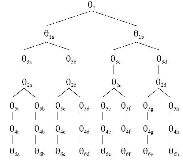
For a Puma arm, there are four possible solutions for the first three joints. Each of these solutions has two possible solutions for the last three links, as shown in Figures 8 and 9. In order to be able to choose the desired of these solutions, we introduce some indicators depending on the setup of the arm, which are translated into signs (+ or -) for the equations. These indicators are determined according to the arrangement of the members (hands) of the human body, and in particular, the position of the shoulder, the elbow and the wrist, and are as follows.
Shoulder Right: +1 | Elbow over wrist : +1 | Wrist down: +1
Shoulder Left: -1 | Elbow under wrist: -1 | Wrist up : -1
The Graphical User Interface. Additions, Changes, Improvements
Several changes were made to the original code, increasing its functionality. The main ones are
- Ability to fully solve the inverse kinematics problem,
- Display Denavit-Hartenberg parameters
- Display the final 06T transform matrix
- Enhance graphical interface capabilities
A breakdown of the changes and additions is given below.
Inverse Kinematics Solver
In the original code, there was a function called PumaIK, with a limited ability to solve the inverse kinematics problem. The solution was incomplete as only Inverse Position Kinematics were resolved and no solution was provided for Inverse Orientation Kinematics. Also, at most one solution to the inverse problem was returned without the option of changing it. Finally, the user could use this function. Extensive changes were made to the PumaIK code. Existing equations were corrected and those missing were added to match those developed in the previous section. Functions were also added to find more solutions.
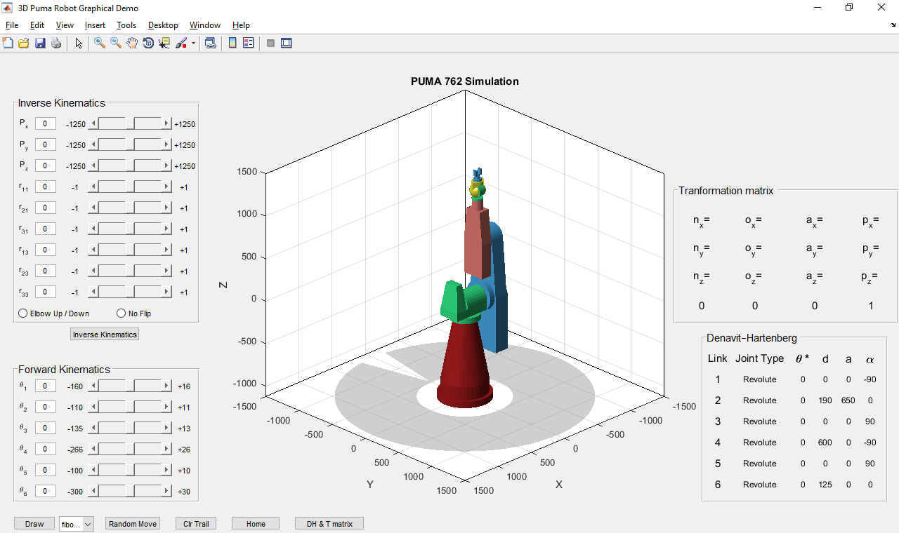
The Inverse Kinematics table was added to the graphical interface so that the user could enter the position and orientation values of the desired end position. It is possible to input the nine variables (Px, Py, Pz, r11, r21, r31, r13, r23, r33) needed to find the final position of the endpoint in the Inverse Kinematics table. The input can be done in two ways, by entering the value in the corresponding field or by changing the slider bar as in the Forward Kinematics table. To the left and right of each slider bar are the minimum and maximum values that each variable can receive and each input is controlled by the check_edit function. Below the input fields, there are radio buttons where the user can choose which solution to the problem they prefer. Specifically, the first radiobutton gives the option of preferring the solution where the elbow is up or down in the final arm assembly with the elbow up being the default device. The second radiobutton offers the choice of rotating or not the end element.
Display Denavit-Hartenberg parameters and final 06T transform matrix
Another important addition is the ability to display the Denavit-Hartenberg parameter and especially the final 06T transform matrix. Although their role is auxiliary, they give an educational tone and complement the graphical environment.
The Denavit-Hartenberg parameter table displays the parameters of each link of the robot. In the Transformation matrix table, we can see all the values of the homogeneous 06T transformation. Many times these values can be used to verify and correlate the solutions of the two kinematics problems, but not always as the inverse solution is not always unique.
A button (DH&T matrix) was implemented in the graphical interface to show or hide these two tables.
Enhance graphical interface capabilities
Another change made to the GUI is replacement the Demo button with the Draw button. This is not just a name change. The name change was made to highlight its functionality. Right next to it a drop-down menu was added to allow the user to select one of the five different drawings. Of course, besides the name and addition of the menu, there was a big change in the code. So with the push of the Draw button allocated function checks which of the drawings is selected and proceeds to its design.
For each design, there is a matrix of values in the 3D space of each point that constitutes it. These matrices were created with the help of GeoGebra software. The function takes these points one by one and passes them to the PumaIK function. In turn, PumaIK calculates the angles that the robot links need to form so that it can be found at that point and then sends them to the pumaANI function with the option 'track trace' enabled. Thus each point of the drawing is highlighted in the 3D space with a blue dot whose whole constitutes the final drawing.
Other minor changes include the addition of a grid to the axis of the arm to facilitate the verification of the right position, but also the activation of the graphical interface window menu whose different tools make it easy to study the robot's motion. For example, the "Rotate 3D" tool allows the axes to rotate giving a better perception of the robot even from angles that initially are considered "blind spots". Finally, appropriate changes were made to make the graphical interface look the same on all systems, regardless of the size of the screen on which it is displayed.
Conclusion
In this project, we managed to create a graphical interface that allows the user to study the Forward and the Inverse Kinematics Problem for one of the most widely used robotic arms. Using the foundations that Don Riley had put in the original code, we took the project one step further, paving the way for further improvements to the utility of the code.
Bibliography
- Craig, J. J. (1985). Introduction to Robotics, Mechanics and Control. 3rd Ed.
- Cubero, S. (2007). Industrial Robotics: Theory, Modelling and Control.
- Dolinsky, J.-U. (2001). The Development of a Genetic Programming Method for Kinematic Robot Calibration.
- Robot Manipulators. Position, Orientation and Coordinate Transformations. (n.d.).
- Spong, M. W., & Vidyasagar, M. (1989). Robot Dynamics and Control 2nd Ed.
- Unimation. (1986). PUMA_761_762_Equipment_Manual.
- Ziegler, C. s. (1983). Geometric Approach in Solving Inverse Kinematics of PUMA Robots.
- Emiris, D. (2004). Ρομποτική.
- Boutalis, Ι. (2014). Διαλέξεις Ρομποτικής.
