CrazySLAM Save
SLAM algorithm with ultrasound range input implemented on a Crazyflie drone
CrazySLAM
CrazySLAM implements a SLAM algorithm using ultrasound range inputs to localize the Crazyflie drone. The project was conducted as part of my engineering degree at INSA Rouen Normandie.
Some background
The localization stack is the most important module in autonomous, mobile systems. Where in some cases the solution to this problem is pretty straightforward (applications with a high inaccuracy tolerance and high prior knowledge of an outdoor environment), it can get really difficult for some kind of devices.
One of the biggest challenges in localization is when the vehicle is operated in an indoor environment. Because it can't use GPS sensors, some of the remaining options are :
- Using cheap/inaccurate sensors (mainly IMUs) but they tend to drift, which could lead to huge errors.
- Using high-end sensors (high precision IMUs, LIDAR, depth cameras, etc.) which are accurate but needs significantly more processing power and can't be implemented on a small-sized vehicle.
- Using prior knowledge of the environment (map, set points), which is a good idea only for very specific applications (robot in a warehouse).
None of these options were good enough for the Crazyflie:
- The Crazyflie framework uses IMUs with a Kalman Filter but the position is inaccurate and tends to drift even more.
- High end sensors can't be implemented on such a small scale drone: Not powerful enough to lift a heavy sensor. Batteries not powerful enough to sustain a heavy load. Not enough processing power onboard. Radio bandwidth not big enough for large high frequency data transmission to a ground station.
- Could use the Loco Positioning system but doesn't scale as you need to install it in the environment where the drone will operate.
SLAM algorithms
Simultaneous Localization And Mapping (or SLAM) is the computational problem of constructing the map of an unknown environment while simultaneously updating the position (or state estimate) of the vehicle. This is what a SLAM algorithm generally looks like:
- Given sensors observations at t-1, construct/update the map
- Estimate the position of the vehicle at t (using a motion model for eg)
- Correct the position estimate given sensors observations at t and the map at t-1
In others words, the intuition behind this class of algorithms is : What motion best explains the difference between sensors observations at t-1 and t given what is known about the environment ?
To implement this method on the Crazyflie, a Kalman filter state estimate is used (for step 2) which is computed by the drone's firmware. It uses sensor measurements from the onboard IMU and gyroscope. For map updates and to correct the state estimate (step 1 and 3), the Multi-ranger deck that has 6 TOF ultrasound sensors is used.
Implementation
Currently, the implementation only supports 2D localization. The state vector contains the position along the x axis, y axis, and the yaw (or heading).
Mapping
The map is represented as an occupancy grid. It's a 2D array where the value in the (i, j) cell is the probability of it being occupied. But keeping track of probabilities directly can be hard (because of some mathematical constraints). Instead of using occupancy probability, the occupancy log odds are used.
The odds of an event are the ratio of the probability of the event happening over the probability of the event not happening. Because of the characteristics of the log function, the computation for map updates then becomes additions of the log odds.
The update rules for a cell in a 2D grid map are :
- Occupied cell :
grid[i, j] += LOG_ODD_OCC - Free cell :
grid[i, j] -= LOG_ODD_FREE
The values of the log odds (LOG_ODD_FREE and LOG_ODD_OCC) will be fixed
parameters of the model. We'll clip the log odds values to minimum and
maximum values (LOG_ODD_MIN and LOG_ODD_MAX which will also be parameters)
as it's never good to be too sure about a cell being occupied or free.
With this representation, the update algorithm becomes relatively simple:
- At each timestamp, use the position estimate and the range observations to find the target (point where the range is measured).
- Compute the index coordinates of those targets in the map. These are the occupied cells since the ultrasound beam was reflected on them.
- Compute the index coordinates of all the cells in the path of the sensor "beam" using the Bresenham line algorithm. If the ultrasound beam was reflected on the targets, it means that it traveled between the target and the vehicle. Which is only possible if the path is unoccupied (i.e. cells along this path are free).
- Apply the corresponding update rule for each kind of cell
Results
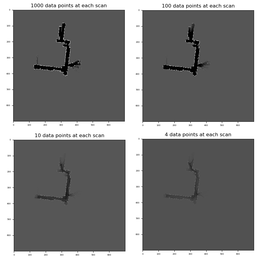
The following simulations use data from the course on robotics by the University Of Toronto on Coursera.
The data is a set of LIDAR scans from a moving robot with accurate state estimations. On the following figures, the environment is mapped using 1000, 100, 10, then only 4 LIDAR points from each scan. This is to demonstrate the loss of information related to a smaller number of data points (only 4 TOF sensor are used on the Crazyflie).
Performance
The implementation of this module is fully vectorized, which allow high frequency map updates. The following frequencies were measured using an Intel Core i5 CPU, with 8 cores.
| Number of data points in each scan | Update frequency |
|---|---|
| 1000 | 50 Hz |
| 100 | 400 Hz |
| 10 | 1200 Hz |
| 4 | 1400 Hz |
Localization
The localization module answers the question that was asked earlier :
What motion best explains the difference between sensors observations at t-1 and t given what is known about the environment ?
Because we use inaccurate sensors, there is a lot of noise in the state estimate. A Particle Filter models this noise with a Gaussian representation. Instead of keeping only one state estimate, it use a big number of particles, with every particle representing a possible state of the vehicle with a corresponding weight (the bigger the weight, the most likely the particle represents the ground truth state).
At each timestamp, it looks at the sensors range inputs and the map. To update each particle's weight, it computes a correlation score : Given the position estimate of the particle, is there any compatibility between what the sensors "see", and what they're supposed to "see". In other words, are the targets on the sensors observations occupied cells on the map.
Algorithm :
- Propagate the particles using a motion model (with observations from the sensors)
- Add random noise to differentiate the particles
- Update the particles' weight by computing the correlation score
- Particle with the highest score becomes our current state estimate
To ensure that all the particles are still relevant, the particles are re sampled at the end of each iteration if the number of effective particles is lower than a fixed threshold.
Results
The following simulations also use the Coursera's data. Because it don't contain any IMU or odometry readings for the motion model update, we'll just use random walk.
On the next figures, the state estimates are made using a fixed number of data points on each scan but a variable number of particles
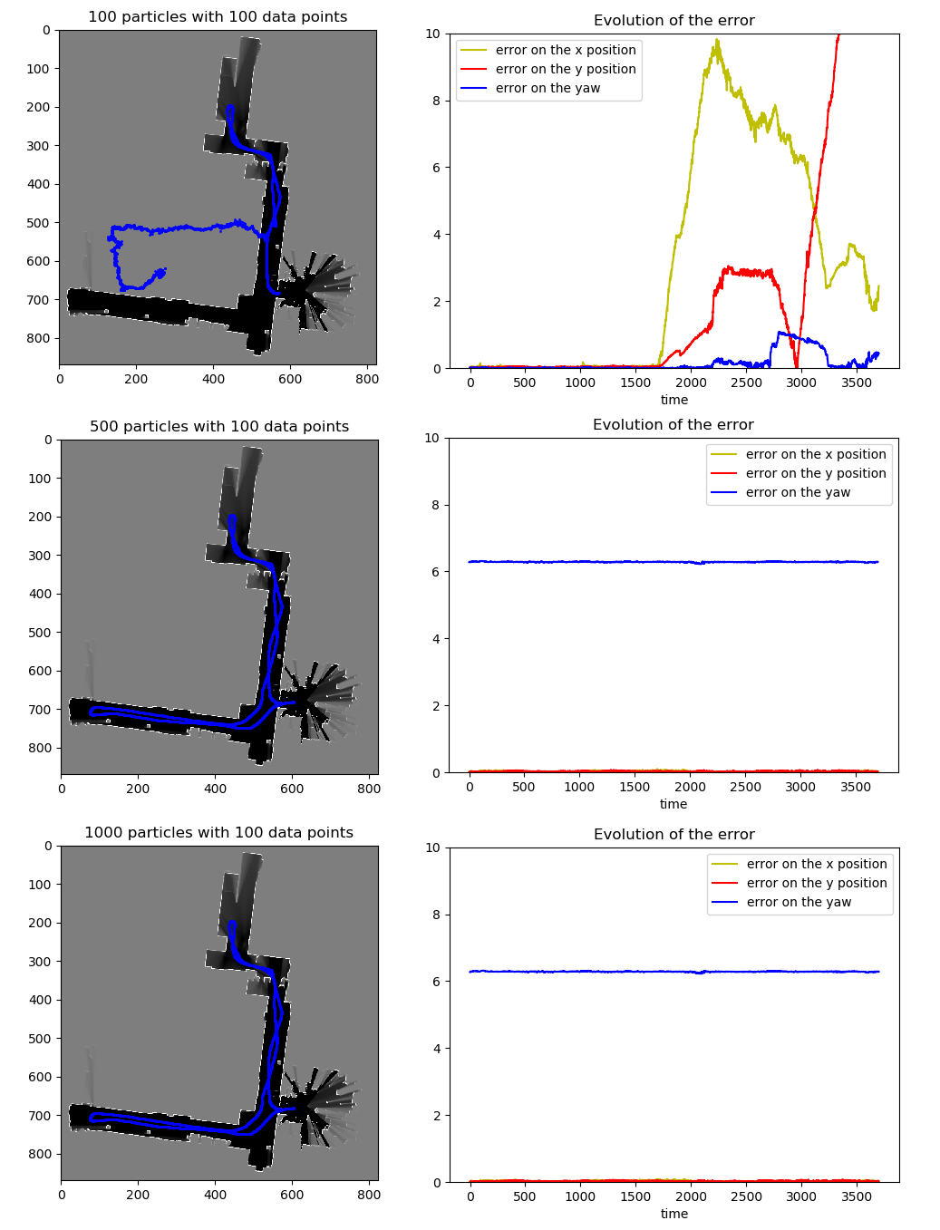
With a small number of particles, the algorithm seems to get lost along the way. The fist half positions are accurate but then the error grows exponentially. The downside of using random walk is that it involves a lot of luck. This will not be a problem for our implementation as we'll use the state estimate given by the onboard Kalman Filter algorithm.
With a big enough number of particles, the error is nearly non existent.
On the next figures, the state estimates are now made using a fixed number of particles but different numbers of data points on each scan.
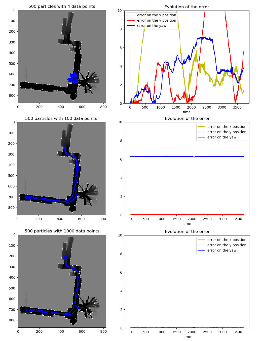
With just 4 data points on each scan (what is available on the Crazyflie), the algorithm performs badly and don't seem to find the correct path with 500 particles.
The experiments showed that it is not the case with a bigger number of particles (+1500), but this poses another issue : performance.
Performance
The previous simulations gives us the following performances :
| Number of data points on each scan | Number of particles | Update frequency |
|---|---|---|
| 100 | 100 | 740 Hz |
| 100 | 500 | 180 Hz |
| 100 | 1000 | 13 Hz |
| Number of data points on each scan | Number of particles | Update frequency |
|---|---|---|
| 4 | 500 | 360 Hz |
| 100 | 500 | 180 Hz |
| 1000 | 500 | 25 Hz |
Putting it all together : SLAM
Given the two previous modules, the SLAM algorithm is quite simple:
- Update the grid map using the current state estimate
- Propagate the particles using the motion model
- Update the state estimate using the Particle Filter
Results
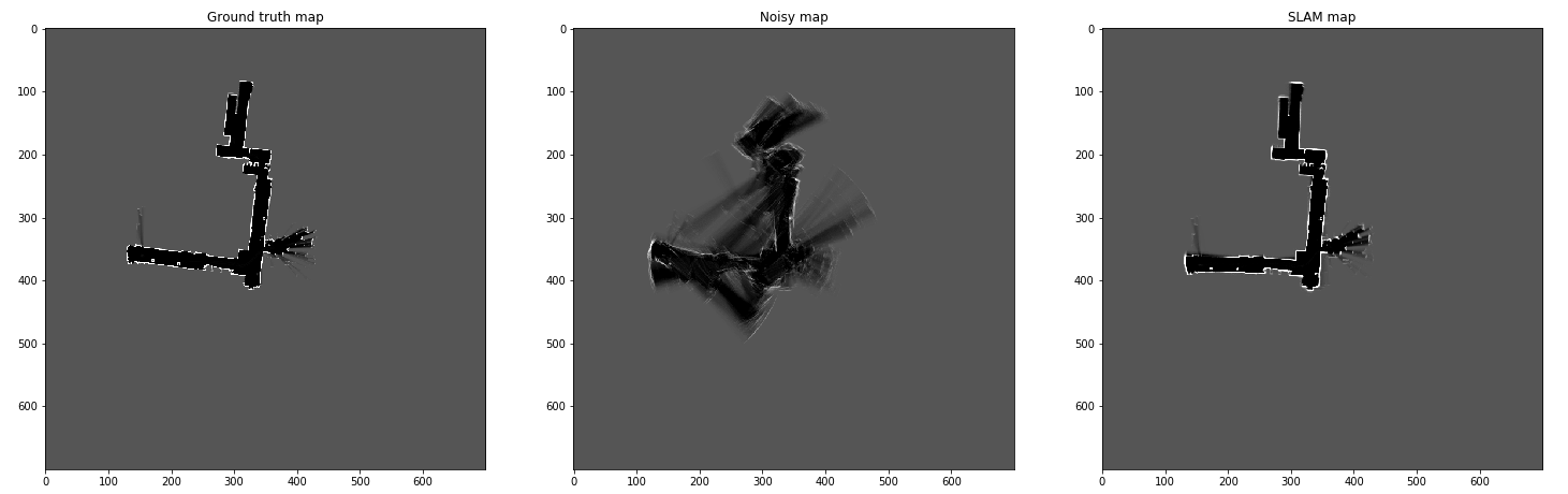
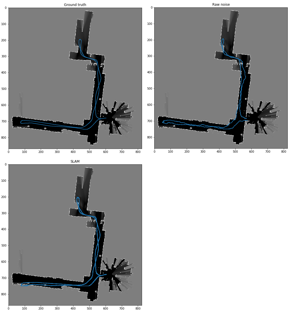
The first set of figures shows the ground truth map on the left, the map with
noisy state estimates in the middle and the one with the SLAM algorithm on the
left.
We see excellent results for the SLAM algorithm, even though the orientation is
skewed anti-clockwise.
The following figures shows the path plotted on the ground truth map.
The path is correct but seems to be off on the lower side of the map.
Finally, the error analysis (difference between the slam state vector and the
ground truth) shows that globally the SLAM algorithm succeeds at correcting the
state estimations :
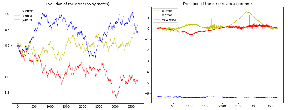
- The yaw correction is perfect
- The x and y estimations may be a little bit off sometimes but the algorithm always seems to converge to the correct state estimate.
The biggest problem however is performance. The previous simulation ran with 3000 particles and 1000 data points and took around an hour. With an update speed of only 3 Hz, it can't (for the moment) be used in real time.
Install
git clone https://github.com/khazit/CrazySLAM.git
cd CrazySLAM
pip install .
Contributing guidelines
- Mapping module:
- Vectorized implementation of the Bresenham line algorithm for multiple targets
- Use a field of view representation instead of a straight line for the ultrasound path (see Extending the Occupancy Grid Concept for operators for example)Low-Cost Sensor-Based SLAM)
- Post processing on the map in between iterations (edge detection operators ?)
- Localization module:
- Compute the correlation score using the occupied AND the free cells
- Implement dynamic noise (current implementation use fixed covariance values for noise generation, whereas noise is proportional to the speed of the vehicle)
