comma-speed-challenge

Project Overview

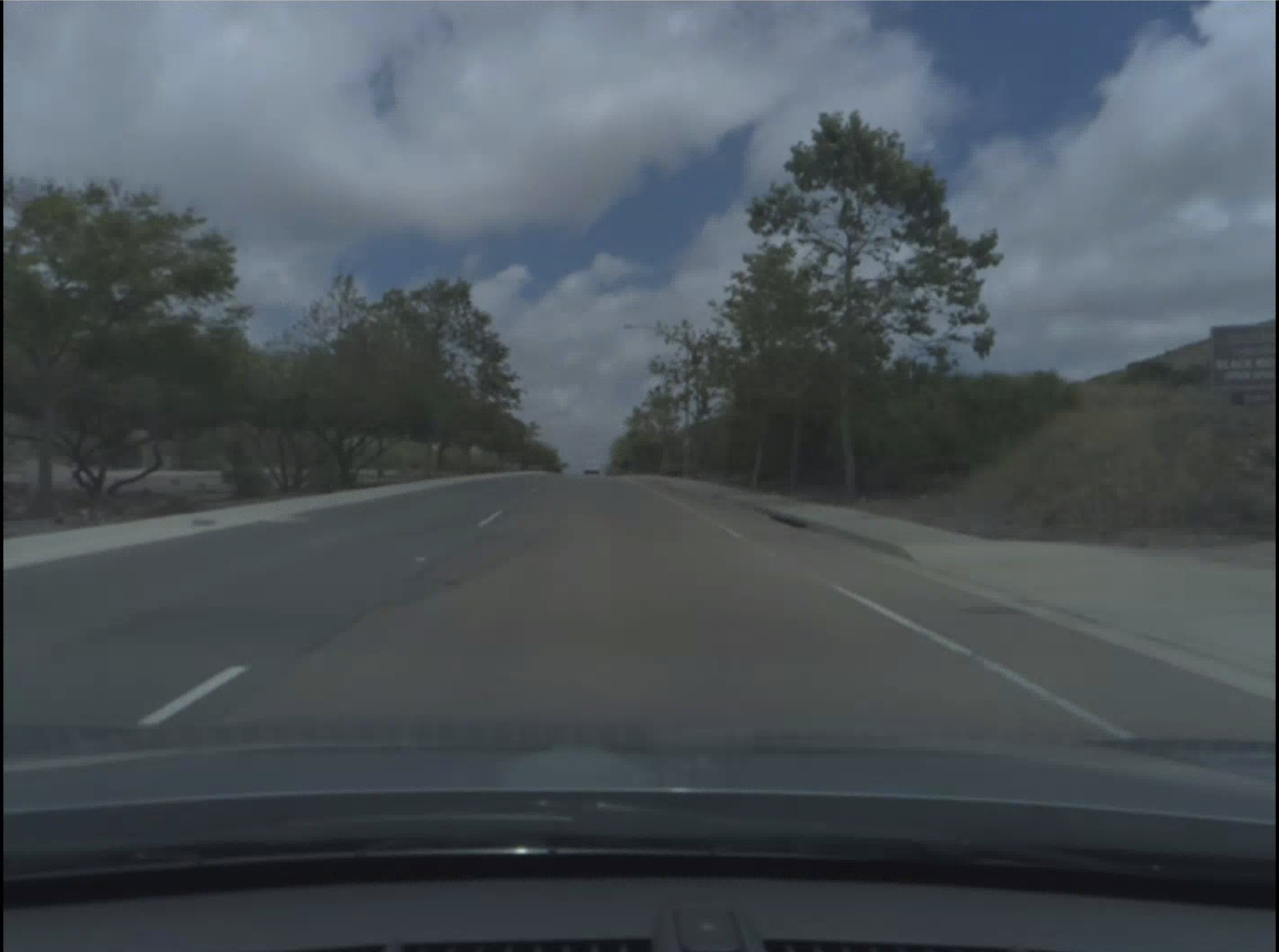
In this project I'll be doing a deep dive into the Comma Speed Challenge. The goal of this challenge is to be able to accurately predict the speed of a vehicle given dash cam footage. I built on top of previous solutions and added significant contributions in the way of creating a data gathering and cleaning pipeline that converts raw data from the EON device to the speed challenge format as well as improving upon previous validation techniques.

Files of interest

• data_pipeline.ipynb
• kfold_models.ipynb

Scratch Files(Experiments that were abandoned)

• CNNLSTM.ipynb (Used to test various architectures and generator setups)
• data_to_hdf5.ipynb (Used to prototype data handling process)
• first_log_frame_reader.ipynb (attempt at using frame reader to pull individual frames from raw .hevc. Abandoned due to speed)
• learning_order.ipynb (Experiment trying to order frames after a shuffle)

Ports to python 3 and tweaks

• Cereal
• Openpilot_tools

Data Location

• train_data (Comma)
• test_data (Comma)
• custom_data (Self-collected)

Outline

1. Background Research

   • Prior speed challenge work
   • Video classification

2. Experiments

   • Full-fat CNN-LSTM
   • 224-224 transfer learning
   • Optical-flow CNN-LSTM
   • Optical-flow flattened CNN
   • Learning frame ordering
   • Crop and Op-Flow flattened CNN

3. Data Gathering

   • Extracting files
   • Identifying data of interest
     • .hevc
     • .rlog
   • Extracting data from files of interest
     • Struggles with Capnp on Mac
     • Docker Attempt
     • Ubuntu VM on Windows
     • FFMPEG
     • Log Reader port to Python 3
     • Resampling Speed
     • Op-flow
     • Augmentation
   • Results
     • Data Quantity
     • Formatting
     • HDF5 Array

4. Data observations

   • Bi/Tri-modal Speed distribution
   • Varying brightness
   • FFMPEG compression aberations
   • ~24fps vs 20fps
   • Frames less frequent than .rlogs

5. Transferring to Comma Data

   • Generalization

6. Validation Strategies

   • Shuffled train-test split
   • Unshuffled train-test split
   • Unshuffled K-folds

7. Final Results

   • Robust Classifier built with new data
   • Comma Data Fine-tuning

8. Path to improvement

Background Research

Going into this challenge I already had several techniques in mind. The approach I imagined would be most successful was a Conv-LSTM in which the convolutions would simplify the image information down into a vector and then the LSTM would iterate through the vectors in order to understand the temporal aspect of the video.

I had read this blogpost previously on video classification and had seen the performance comparisons and figured I could likely transfer many of the techniques and convert the task to regression relatively easily. Another tool I pulled out was h5py in order to store the data as a large array that I could quickly access. My prior experience has shown that this is highly favorable when dealing with images. In this specific challenge I don't know that I procured as much gain as in previous projects though. In the past I had a challenge with 1+ million jpegs and I believe the issue was seeking all of the individual files. Due to the relatively small number of frames this was not as big of an issue.

Prior speed challenge work

With this knowledge in mind I went to look at what had already been done on this challenge. I gathered any reputable sources and reviewed techniques that seemed to be successful.

• https://github.com/JonathanCMitchell/speedChallenge
• https://github.com/satyenrajpal/speed-prediction-challenge
• https://github.com/Quantzz/commaai-speed-challenge
• https://github.com/yangarbiter/commaai-speed-challenge
• https://github.com/jovsa/speed-challenge-2017
• https://medium.com/weightsandbiases/predicting-vehicle-speed-from-dashcam-video-f6158054f6fd
• https://github.com/praateekmahajan/predict-speed-using-dashcam
• http://prtk.in/blog/predicting-speed-of-vehicle-using-dashcam/
• https://github.com/justinglibert/speed-challenge
• https://github.com/graceyang406/speed_challenge
• https://libraries.io/github/experiencor/speed-prediction
• https://github.com/dlpbc/comma.ai-speed-challenge
• https://github.com/djnugent/SpeedNet After reviewing these various sources a few prevalent techniques became apparent:
  • Optical flow was used in order to gauge motion between two frames. This seemed to be a significant differentiator in terms of performance. Multiple people reported poor performance on raw image input. This was confirmed in later experiments. I believe that this may no longer be the case if more data was introduced. The primary issue was likely the sparsity of inputs and over-fitting on minute details present in the raw images of the training data.
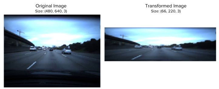
  • Cropping down to the specific areas of interest instead of keeping the whole frame seemed to be valuable. This was highly useful to prevent fitting on scenery instead of the actual movement along the road and also greatly reduced computation and storage required. Many people took the source video from 640x480 down to 66X220 or other lower resolutions
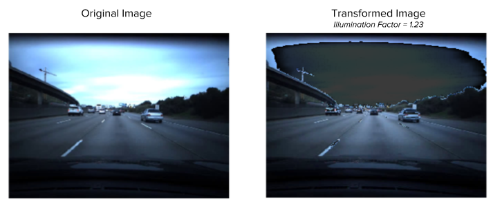
  • Brightness augmentation was utilized in order to fight overfitting. This prevented the network from simply looking for brightness characteristics and hopefully allowed the network to generalize to different conditions. This area seems understudied and could likely be taken further.
  • Single frame optical-flow CNN
  • Multi-frame optical-flow CNN-LSTM or 3D CNN
  • Rolling mean of predictions also showed signficant boost in terms of validation loss. This smoothed the predictions and prevented erratic prediction errors, but also delayed predictions from reaching accurate predictions for a few frames
  • Poor validation techniques : It seems like almost everyone opted for either a shuffled train test split or a unshuffled train test split. I believe that neither of these are strong validation techniques given the temporal nature of the data and small sample size, but I will cover this in more detail later

Video Classification

After doing some experimentation of my own and looking through the prior work I also looked through arxiv.org and various other research focused sites like https://paperswithcode.com/sota in order to see if there were any other major advances that could be implemented here. Papers with code specifically exposed me to the various video focused areas of study. I found there are strong parallels between 3d medical imaging and video classification and regression and also dove into more detail on the datasets referenced in the prior medium blog. Kinetics and UFC101 both looked to be decent baselines for looking at performance of video classification models so I inspected the various models that were being applied to these. In this search I located a relatively comprehensive guide on video techniques http://blog.qure.ai/notes/deep-learning-for-videos-action-recognition-review

This covered performance review of several of the different techniques and variations I had been considering and some I had not thought of. The most promising technique appeared to be one of using Two stream inflated 3D convolutions with imagenet and kinetics dataset pretraining.

Another interesting area that was uncovered was the various methods of optical flow. The dense and sparse method available in OpenCV were both good but there were also a few papers related to CNN based methods for optical flow https://paperswithcode.com/paper/a-fusion-approach-for-multi-frame-optical. This was not further studied but it would be interesting to see if a more precise or faster optical flow calculation would possibly allow for more accurate speed estimates or a real-time implementation.

Two other areas I briefly looked over were methods of pretraining due to the relatively small size of the data. One http://news.mit.edu/2018/machine-learning-video-activity-recognition-0914 method I thought might be useful was inferring missing frames. In the process of predicting what the inbetween frames should be it would likely learn how lane lines and surrounding objects are expected to move. A model could be pretrained on this auxiliary task and then the decoder could be cut off and fine-tuning done on the original task.

Another method for pretraining was learning the ordering of frames. My intuition behind this was that I could likely shuffle the frames of the video going into the network and have it learn the relative order. In this way it would learn the directionality of the movement and begin understanding the expecation that lane lines should be going towards the car in successive frames. After some failed experiments and discussion with colleagues I was pointed towards this blog on pointer networks and learned that sorting via NN was likely not going to be a fruitful endeavor.

Experiments

Some experiments have quantitiative numbers but many were not stored because they were done early in the prototyping phase just trying to debug various approaches and may have been ended prior to convergence

The first experiment that was completed was simply trying to train a CNN-LSTM over a sequence of frames and predicting the speed for the last frame. This was done on the full 640x480 images. This limited the experiment to a relatively short history size of only a few frames. This resulted in lackluster performance. Various tweaks and architectures were attempted but ultimately it did not seem like this approach would be fruitful as was also found in the other attempts at this challenge. A couple backends were applied to this approach. RNN and simple flattening of the output from the time-distributed CNN's. It appeared that the flattening was more successful than the RNN approach. This likely would not be the case if a longer sequence of frames was passed in. 3-4 frames of history is likely not enough to procure a benefit.

Underwhelmed by these results I reviewed a few other approaches like downscaling the images to 224x224 and then doing a time-distributed inception pretrained network but results on this were still not up to par. I started moving to a hybrid approach where I had two pathways, one for the original image and another for the optical flow. In order to measure usefulness of both branches I tried holding out each and found that the image branch was actually detrimental to performance so eventually just dropped the source images and was focusing only on the optical flow images. With these having a reduced resolution I was able to do a longer history. I tried numbers ranging from 16 down to 1 and with varying batch sizes. It seemed like the benefit of increased frame history was not worth the additional computation cost and required smaller batch sizes so eventually I settled on single frame optical flow. This allowed for much faster prototyping and iteration while maintaining performance.

Utilizing downscaled optical-flow images seemed to achieve good metrics, but I wanted to take things beyond what others had done in previous work so I looked into the various pretraining methods at this point. I set up the experiment for learning frame ordering, but even with simple 3 frame shuffles it was not able to learn the ordering. I tried with varying lengths, but the model consistently converged to the middle case. I set this up such that the output of the network was the indexes of the frames. I.e. (4, 1, 3, 2, 0) if it was a 5 sequence length. In this 5 sequence case all outputs would eventually converge to 2 since it is the middle case. There is likely some additional method to make this work better. I reviewed various papers and it looks possible, but did not pursue it further without an easy path forward.

After these failed attempts to improve upon prior work I realized one of the most major problems I was seeing with my models I was toying with was instability and inconsistency. It seemed like gathering additional data or augmenting what was provided was the way forward to create a model that was more consistent across epochs and had a greater chance of generalizing to the test set.

Data Gathering

Realizing the benefit of more data I began to record drives and work through a process in order to extract data from my eon in a similar format to what was provided for this challenge. There were a few key hurdles I had to overcome here. First, the frame-rate was different than what was provided, I did not know of a method to extract the cars readings, once I did extract the rlogs and hvec files they were not synced in terms of polling rates.

I figured out how to extract the files from the eon via the wiki and directions off of opc.ai, but still needed to figure out how to match the formatting of the speed challenge video and speed readings.

I initially did this manually by taking each 50 second .hevc clip stored on the eon and passing them through handbrake with equivalent settings. I discovered that the source resolution was higher and needed to be scaled down to 640x480 and also that the frame rate was ~24 instead of 20 like in the video provided to us. After some tweaking and tuning of the handbrake settings I was able to create videos that looked visually similar.

Now that I had the video in an equivalent format I needed to make the speed readings match up. I had a huge hassle with originally opening up the .rlog files. I took a few stabs at simply opening with python with various encodings, but didn't find anything that seemed to make sense. Eventually I looked through the various Comma repo's and discovered the https://github.com/commaai/comma2k19/blob/master/notebooks/raw_readers.ipynb file which shows the reading of both the logs and frames, but relies on the https://github.com/commaai/openpilot-tools repo being installed.

I attempted to get this running on my Mac in various different ways, but ran into several dependency issues. Eventually I ran across the main culprit, capnp and the associated error on github https://github.com/capnproto/pycapnp/issues/177. I tried the various fixes, but did not have success with getting capnp installed on Mac so I looked at various other resources and eventually just settled on setting up an Ubuntu VM on my windows box. With this I was able to install all of the various Comma related dependencies relatively easily.

From here I ran into another issue, all of these tools were based on python 2.7 so I removed any python 2.7 specific dependencies and replaced them with python 3 equivalents like changing subprocess32 to subprocess and swapping out print statements with print(statements) and xrange with range. Now I was able to read in the log files as well. I discovered these didn't quite line up with the frame counts though so I needed to create a resampling function that would take in the number of frames per the video and make the received speed readings match that timeframe.

Eventually I got both the videos and speed readings what seemed like a reasonable format and model performance seemed to roughly be working so I worked on automating the process a bit more. I created the data_pipeline.ipynb which is able to convert the source video to the correct format via a subprocess call which converts with ffmpeg. From there the number of frames is returned and the log files are loaded in and rescaled to match the video length. Then optical flow and augmentation are applied and these files are stored in hdf5 array for quick and easy reaccess in the future. The frames, optical flow and speed readings are all stored in parallel hdf5 datasets so if the frames are required for model result inspection in the future the frames of high error can be loaded in order to visually inspect conditions where model fails. Doing this directly on optical flow images is not particularly useful.

Various improvements were made after the fact such as automatically moving processed files to a new directory and storing all downscaled videos out of ffmpeg. This turned out to be handy in the case of augmentation changes and recomputing the dataset. One major thing I would go back and change would be the ordering of the videos. I implemented a simple system that cuts off the first two clips and last two clips of each timestamped video in order to prevent any potential privacy issues if I decided to open source the data I have gathered, but I did not bother to write the data in chronological order. This caused the issue of doing the running mean over predictions between two non-contiguous clips sometimes causing unwanted lags or jumps in results between 1000 frame sets.

Results

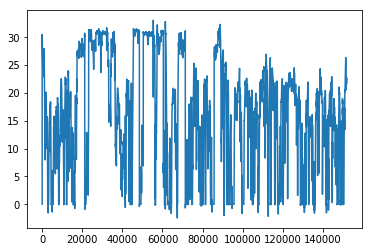
Once this data was gathered across a couple of weeks I was able to gather roughly 150k frames worth of data. This ended up totalling 22.6gb, but could be much smaller if HDF5 compression was turned on and chunking size was altered. I opted not to do this since it would negatively affect read time and the array isn't ultimately that big. Ultimately I think there is still much to be desired in terms of data gathering. I considered the possibility of saving each clip as their own independent HDF5 dataset in order to prevent the rolling averaging errors or allow for some other form of shuffling and on the fly augmentation, but it wasn't a huge priority since the current method seemed to work reasonably well despite the various areas of improvement.

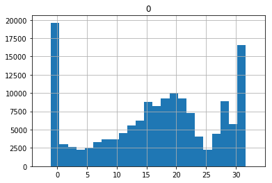
Data Observations

Throughout the project several observations were made about the data. The first being that it seems like the data will end up being trimodal. This is because cars really have three modes.

1. Stopped
2. Highway driving
3. Non-highway driving There are peaks at the speeds of these modes, but you can see that these numbers are slightly different between the data I gathered and the data provided by comma. It seems like the driving I was doing through areas with lights rather than stop signs caused me to be stopped for much longer periods and my speed on the highway was higher.

Comma Data Histogram

Custom Data Histogram

This brought about a couple thoughts. Because the data has these long stretches of the car at these three modes but relatively more sparse examples of accelerating and decelerating between these modes it might be fruitful to oversample the data in these less common scenarios. This was not acted on or experimented with but it was considered.

The other things that were noticed about the data was the difference between brightness. Most of the driving that I was able to capture was around lunch time or other times of high brightness but the driving from the training data appears to a much lower brightness time of the day. It likely would have been useful to do more dusk/dawn driving in order to get a closer match.

Another area that was slightly different was the conversion done by ffmpeg. I wasn't sure about the method that was used for the training video and after inspection it looked like the compression by default in ffmpeg was likely causing some aberations. It is hard to say if these would have caused issues but the compression was apparent in the video and I didn't want these artifacts to transfer to the optical flow calculation so I changed the compression rate to be nearly lossless.

Frame rate and method for downscaling the log readings were also considered but those seemed to work reasonably well. FFMPEG was able to automatically convert the frame rates between the two values and based on the outputs it seems that it was simply dropping every fews frames because it was printing a metric for dropped frames. I figured this was likely better than doing some reaveraging between frames that may have caused some smearing or ghosting.

Transferring to Comma Data

Given the various differences in the data I gathered against what comma provided there was some concern of whether the model trained on this data would generalize. To see if this would work I tried training solely on the custom data and then validated on the comma provided data. This did surprisingly well.

At this stage I was simply doing a 80/20 unshuffled split and was able to achieve 1.56 MSE with just the custom data alone, single frame history and some smoothing. The second method I tried was alternating epochs between training on the custom data and comma data. This ended up finding a minimum MSE of ~1.8 so it shows that the data does have strong generalization to the new data. On closer inspection though I chose to do the alternating epochs because it seemed to give much more stable results. The custom data alone had much less consistent loss patterns.

One thing I was paying close attention to during the training process was the distribution of predictions. I had to remove batch normalization from the network because it seemed to cause random and erratic spikes in some predictions. All predictions would be reasonable and then one or a few predictions would be in the thousands or negative. This was discovered by printing off the predictions distribution after training each epoch.

One other thing that was observed that when training only on the custom data the distribution seemed to be shifted sometimes when doing predictions on the comma data. Very often all of the predictions would be a few M/S low. These graphs made the debate over fune-tuning on the comma data more clear because that seemed to remedy that.

Validation Strategies

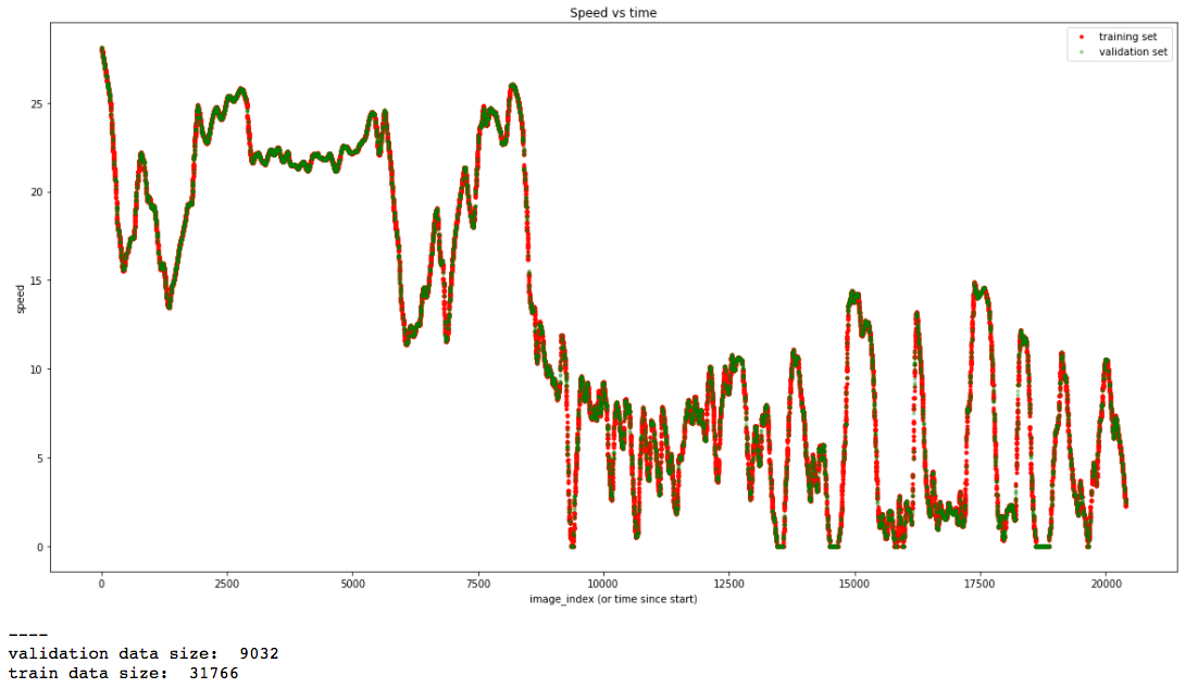
One major thing that I believe people are making a mistake on is the validation schemes they are using for this challenge. Ultimately in my final model I chose to utilize K-Folds. I deemed a shuffled train-test split invalid because it was leaking information to the model. If it saw a frame before and a frame after the frame that was being predicted on it has a signficant advantage over what it will likely be encountering in the wild. Similarlly an unshuffled split was not a good idea due to the various modes of driving. It seems that the final 20% of the data most people were using for validation is primarily slower driving where loss is artifically depressed do to the condensed range. 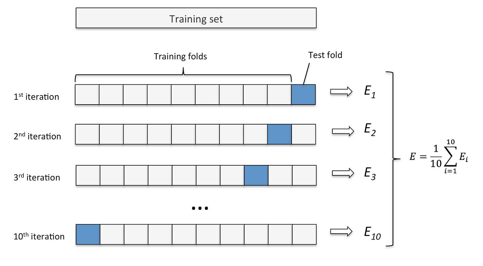Because of these two reasons I think k-fold and training models on each of the folds is the only way to get a successful representation of what future performance will look like on unseen data. This is a little bit tricky since I am dealing with training on two independent datasets. I chose to do k-folds on both of the datasets at the same time so I could gauge performance on the custom validation and the comma validation, but I believe performance likely would have been better if I trained on the entirety of the custom data and only the folds of the comma data. Another combination I considered but deemed unreasonable was one k-fold over the comma data and another around the custom data, but this would have required potentially 25 models to be trained for a 5-fold setup.

Final Results

With all of these things in consideration I was able to create a model that achieved MSE of 5.06 on the comma data and 8.25 on the custom data. This is good but not amazing. It is difficult to say if this will have greater generalization capability than the prior methods listed in the background research section, but I do believe these numbers are likely closer to reality than those mentioned in many of the previous works stating numbers as low as 1.1 MSE. The novel contribution in this work is not a model improvement but a data improvement and process improvement. In the below section I will state how this number can likely be driven lower.

Path to Improvement

There are many things that still have large room for improvement. Obviously more data wouldn't hurt but I believe that will eventually reach diminshing returns when only being captured from one device. Performance would likely improve more with a greater variety rather than all of it coming from my one specific installation.

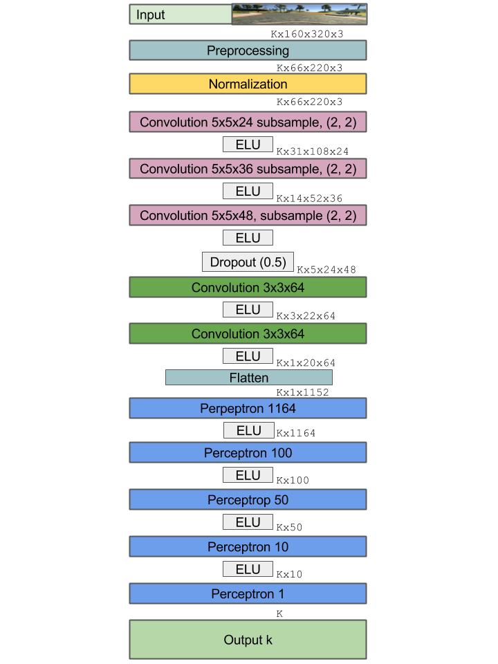
Another area of improvement is the model. The one I put together was simply a two branch convolutional model with 3x3 convolutions and 5x5 convolutions in parallel and max-pooling layers. The final design did not exploit any temporal aspect of the data beyond what was captured by the optical flow. It would likely be fruitful to move to the more advanced architectures like the inflated convolutional 3D network or a CNN-LSTM network. There are likely some longer dependencies that could be captured such as a stop sign or light being a good signal that a speed change is going to occur or familiarity with what a freeway on-ramp looks like being indicative of an impending increase in speed or a system to detect speed signs. These kinds of things are not captured with the optical flow alone so the raw images would likely be valuable as well if more data and longer history sequences could be trained on.

The model architecture and augmentation schemes can be improved and tuned systematically via neural architecture search and google autoaugment. https://towardsdatascience.com/how-to-improve-your-image-classifier-with-googles-autoaugment-77643f0be0c9 Using this it could be derived what angles of variation people apply when installing the device as well as any other variations such as different tints on the windows and the augmentor could simulate these different scenarios.

One of the keys to further improvement is deeper error analysis. One thing I considered but did not get to was making a system that would grade predictions and output the video of the 10 seconds of highest loss and see if there are any areas or patterns to where the algorithm is consistenly wrong and if there is anything I can do with the model or inputs in order to prevent this.