Bayesian Coherent Point Drift (+ Geodesic Kernel)

-- 7 Apr 2023 - A new article was officially published.

This software is an implementation of non-rigid registration algorithms, Bayesian coherent point drift (BCPD) and its faster variant called BCPD++. It also includes geodesic-based BCPD (GBCPD) and its accelerated variant (GBCPD++), which define the shape deformation prior using geodesic distance. The software has the following characteristics:

• Scalability. It non-rigidly registers the shapes containing over 10M points (3M points if geodesic kernel).
• Robustness. It performs non-rigid registration with robustness against outliers and target rotation.
• Multipurpose. It performs rigid registration under appropriate parameters to find the partial overlap between 3D scans.

For more information, see Hirose2022 (GBCPD/GBCPD++), Hirose2020a (BCPD), and Hirose2020b (BCPD++). Also, several examples can be watched in [Video 1], [Video 2], [Video 3], [Video 4]. If you have any questions, kindly email ohirose.univ+bcpd(at)gmail.com with your name and affiliation.

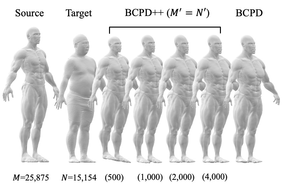
Table of Contents

1. Papers
2. Performance
   • GBCPD vs CPD
   • BCPD vs CPD
   • BCPD vs BCPD++
3. Demo
   • Surface registration
   • Point set registration
   • Shape transfer
4. Compilation
   • Windows
   • MacOS and Linux
5. Usage
   • Terms and symbols
   • Input data
   • Tuning parameters
   • Kernel functions
6. Acceleration
   • Nystrom method
   • KD tree search
   • Downsampling
   • Interpolation
7. Options
   • Convergence
   • Normalization
   • File output
   • Terminal output
8. Rigid registration

Papers

The details of the algorithms are available in the following papers:

• [GBCPD/GBCPD++] O. Hirose, "Geodesic-Based Bayesian Coherent Point Drift," IEEE TPAMI, Oct 2022.
• [BCPD++] O. Hirose, "Acceleration of non-rigid point set registration with downsampling and Gaussian process regression," IEEE TPAMI, Dec 2020.
• [BCPD] O. Hirose, "A Bayesian formulation of coherent point drift," IEEE TPAMI, Feb 2020.
  • The article's supplementary document contains proofs of propositions.
  • Fig. 15 in the print version was accidentally replaced by Fig. 3 during the publication process after the review process. See an erratum correcting the error.
  • In Fig. 2, following Proposition 3, please replace with as follows:

Performance

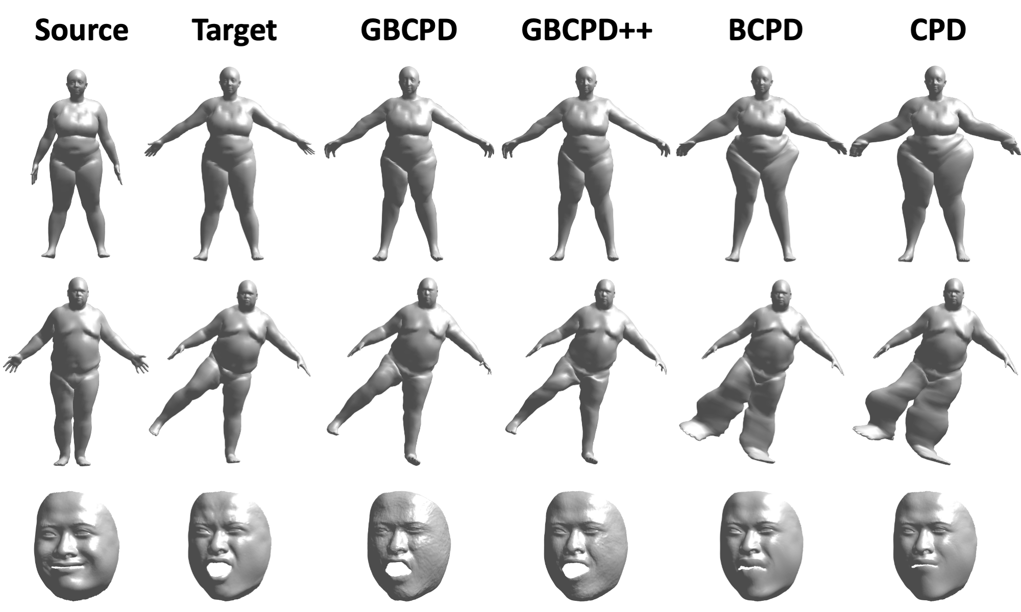
GBCPD vs CPD

GBCPD works better than CPD and BCPD when it aligns shapes with adjacent, different parts, such as left and right legs:

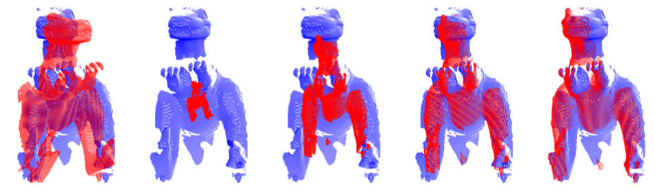
BCPD vs CPD

BCPD is faster than coherent point drift (CPD) and is often more accurate. The following figure shows a comparison using Armadillo data included in demo data (vs Dr. Myronenko's implementation on Macbook Pro Early 2013):

BCPD vs BCPD++

BCPD++ is much faster than BCPD but is slightly less accurate (Mac Mini 2018).

Demo

Surface Registration

• Download the datasets required for demos: GBCPD data.
• Decompress and move the datasets into the data folder in this software.
• Start MATLAB.
• Go to one of demo/[gbcpd/gbcpd++/hierarchy] folders in the MATLAB environment.
• Double-click a demo script, e.g., demoFACE01.m.
• Press the run button in the code editor of MATLAB.

Point set registration

MATLAB scripts under the demo folder will demonstrate various examples.

• Download the datasets required for demos: BCPD data and BCPD++ data.
  • If you have trouble downloading them, go to bcpd-dataset.
• Decompress and move the datasets into the data folder in this software.
• Start MATLAB.
• Go to one of demo/bcpd-[nonrigid/rigid/plusplus] folders in the MATLAB environment.
• Double-click a demo script, e.g., demoFishA.m.
• Press the run button in the code editor of MATLAB.

Shape transfer

Bash scripts under the demo folder will demonstrate Shape transfer/BCPD++ examples without MATLAB. Several examples can be watched HERE.

• Go to the demo/shapeTransfer folder using your terminal window.
• Run a demo script, e.g., type ./shapeTransferA.sh in the terminal.
• Check output files named transferV[1/2]_y.interpolated.obj.

Compilation

Windows

Ready to go. The compilation is not required. Use the binary file bcpd.exe in the win directory. The binary file was created by GCC included in the 32-bit version of the MinGW system. Therefore, it might be quite slower than the one compiled in a Mac/Linux system.

MacOS and Linux

1. Install OpenMP and the LAPACK library if not installed. If your machine is a Mac, install Xcode, Xcode command-line tools, and MacPorts (or Homebrew).
2. Download and decompress the zip file that includes source codes.
3. Move into the top directory of the uncompressed folder using the terminal window.
4. Type make OPT=-DUSE_OPENMP ENV=<your-environment>; replace <your-environment> with LINUX, HOMEBREW, HOMEBREW_INTEL, or MACPORTS. Type make OPT=-DNUSE_OPENMP when disabling OpenMP.

Homebrew's default installation path changes according to Mac's CPU type. If you use an Intel Mac, specify HOMEBREW_INTEL instead of HOMEBREW.

Usage

Type the following command in the terminal window for Mac/Linux:

./bcpd -x <target: X> -y <source: Y> (+options)

For Windows, type the following command in the DOS prompt:

bcpd -x <target: X> -y <source: Y> (+options)

Brief instructions are printed by typing ./bcpd -v (or bcpd -v for windows) in the terminal window. The binary file can also be executed using the system function in MATLAB. See MATLAB scripts in the demo folder regarding the usage of the binary file.

Terms and symbols

• X: Target point set. The point set corresponding to the reference shape.
• Y: Source point set. The point set to be deformed. The mth point in Y is denoted by ym.
• N: The number of points in the target point set.
• M: The number of points in the source point set.
• D: Dimension of the space in which the source and target point sets are embedded.

Input data

• -x [file]: The target shape represented as a matrix of size N x D.
• -y [file]: The source shape represented as a matrix of size M x D.

Tab- and comma-separated files are accepted, and the extensions of input files MUST be .txt. If your file is space-delimited, convert it to a tab- or comma-separated file using Excel, MATLAB, or R, for example. Do not insert any tab (or comma) symbol after the last column. If the file names of target and source point sets are X.txt and Y.txt, these arguments can be omitted.

Tuning parameters

• -w [real]: Omega. Outlier probability in (0,1).
• -l [real]: Lambda. Positive. It controls the expected length of deformation vectors. Smaller is longer.
• -b [real]: Beta. Positive. It controls the range where deformation vectors are smoothed.
• -g [real]: Gamma. Positive. It defines the randomness of the point matching at the beginning of the optimization.
• -k [real]: Kappa. Positive. It controls the randomness of mixing coefficients.

The expected length of deformation vectors is sqrt(D/lambda). Set gamma around 2 to 10 if your target point set is largely rotated. If input shapes are roughly registered, use -g0.1 with an option -ux. The default kappa is infinity, which means that all mixing coefficients are equivalent. Do not specify -k infinity or extremely large kappa to impose the equivalence of mixing coefficients, which sometimes causes an error. If lambda (-l) is sufficiently large, e.g., 1e9, BCPD solves rigid registration problems. If you would like to solve rigid registration for large point sets, accelerate the algorithm carefully; see Rigid registration.

Kernel functions

Standard kernels:

• -G [1-3]: Switch kernel functions.
  • -G1 Inverse multiquadric: (||ym-ym'||^2+beta^2)^(-1/2)
  • -G2 Rational quadratic: 1-||ym-ym'||^2/(||ym-ym'||^2+beta^2)
  • -G3 Laplace: exp(-|ym-ym'|/beta)

The Gaussian kernel exp(-||ym-ym'||^2/2*beta^2) is used unless specified. Here, ym represents the mth point in Y. The tuning parameter of a kernel functions is denoted by beta, which controls the range where deformation vectors are smoothed.

Geodesic kernel:

• -G [string,real,file]: Geodesic kernel with an input mesh. E.g., -G geodesic,0.2,triangles.txt.

  • 1st argument: The string geodesic only., i.e., the tag representing the geodesic kernel.
  • 2nd argument: Tau. The rate controlling the balance between geodesic and Gaussian kernels.
  • 3rd argument: The file that defines a triangle mesh.

• -G [string,real,int,real]: Geodesic kernel without an input mesh. E.g., -G geodesic,0.2,8,0.15.

  • 1st argument: The string geodesic only, i.e., the tag representing the geodesic kernel.
  • 2nd argument: Tau. The rate controlling the balance between geodesic and Gaussian kernels.
  • 3rd argument: The number of neighbors for each node, required for k-NN graph construction.
  • 4th argument: The radius that defines neighbors for each node, required for k-NN graph construction.

The geodesic kernel usually outperforms standard kernels when different parts of a source shape are closely located. If the mesh of a source shape is available, choose the first option; it typically works better than the second option. Otherwise, choose the second option; BCPD automatically creates the graph required for geodesic computations. The mesh file must be a tab-separated file that contains three integers for each line; a triangle is defined as a triplet of vertices. The following parameters tune the geodesic kernel:

• -b [real]: Beta. Positive. Gaussian function's width.
• -K [int]: K tilde. Positive. Rank constraint on G.
• -z [real]: Epsilon. Positive. Acceptable condition number of G.

Acceleration

BCPD can be accelerated inside and outside variational Bayes inference (VBI), separately. The Nystrom method and KD-tree search accelerate VBI. The former works before approaching convergence, whereas the latter works near convergence. The following option accelerates VBI with default parameters:

• -A: VBI acceleration with parameters, i.e., -K70 -J300 -p -d7 -e0.15 -f0.2.

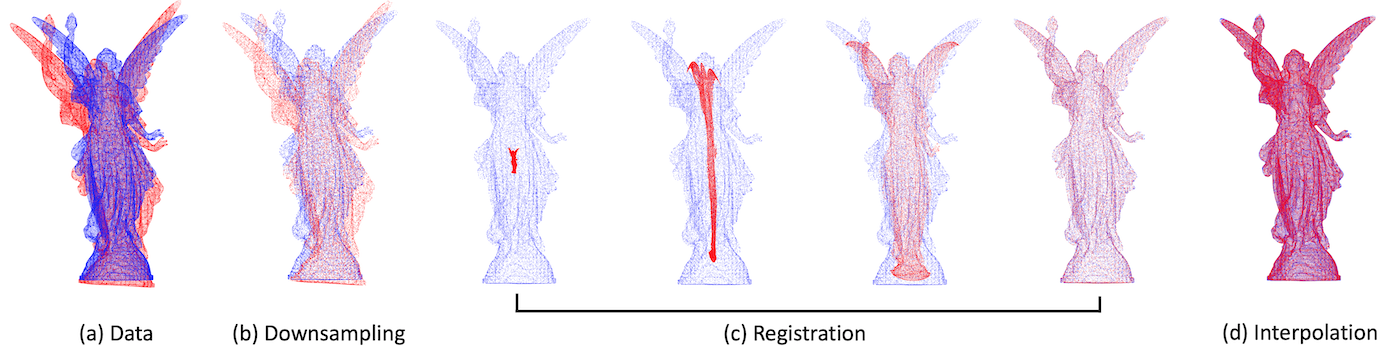
Downsampling and deformation vector interpolation, called BCPD++, accelerate non-rigid registration outside VBI. For example, the following options activate BCPD++:

• -DB,5000,0.08: BCPD++ acceleration outside VBI.

If N and M are larger than several thousand, activate either the internal or external acceleration. If N and M are more than several hundreds of thousands, activate both accelerations. Also, the acceleration methods reduce memory consumption. Either internal or external acceleration method MUST be activated to avoid a memory allocation error for such a large dataset. Otherwise, BCPD sometimes fails without any error notice.

Nystrom method

• -K [int]: #Nystrom samples for computing G.
• -J [int]: #Nystrom samples for computing P.
• -r [int]: Random number seed for the Nystrom method. Reproducibility is guaranteed if the same number is specified.

Specify -J300 -K70, for example. The acceleration based only on the Nystrom method probably fails to converge; do not forget activating the KD-tree search.

KD tree search

• -p: KD-tree search is turned on if specified. The following options fine-tune the KD tree search.
  • -d [real]: Scale factor of sigma that defines areas to search for neighbors.
  • -e [real]: Maximum radius to search for neighbors.
  • -f [real]: The value of sigma at which the KD tree search is turned on.

The default parameters are -d7 -e0.15 -f0.2. Retry the execution with -p -f0.3 unless the Nystrom method is replaced by the KD-tree search during optimization.

Downsampling

• -D [char,int,real]: Changes the number of points. E.g., -D'B,10000,0.08'.
  • 1st argument: One of the symbols: [X,Y,B,x,y,b]; x: target; y: source; b: both, upper: voxel, lower: ball.
  • 2nd argument: The number of points to be extracted by the downsampling.
  • 3rd argument: The voxel size or ball radius required for downsampling.

Input point sets can be downsampled by the following algorithms:

1. voxel-grid resampling with voxel width r,
2. ball resampling with the radius r, and
3. random resampling with equivalent sampling probabilities.

The parameter r can be specified as the 3rd argument of -D. If r is specified as 0, sampling scheme (3) is selected. The numbers of points in downsampled target and source point sets can be different; specify the -D option twice, e.g., -D'X,6000,0.08' -D'Y,5000,0.05'. For more information, see paper and appendix.

Interpolation

Downsampling automatically activates the deformation vector interpolation. The resulting registered shape with interpolation is output to the file with the suffix y.interpolated.txt.

Options

Default values will be used unless specified.

Convergence

• -c [real]: Convergence tolerance.
• -n [int ]: The maximum number of VB loops.
• -N [int ]: The minimum number of VB loops.

The default minimum VB iteration is 30, which sometimes causes an error for small data. If the bcpd execution stopped within 30 loops with an error notice, execute it again after setting -N1, which removes the constraint on the minimum VB iteration. The default value of the convergence tolerance is 1e-4. If your point sets are smooth surfaces with moderate numbers of points, specify -c 1e-5 or -c 1e-6.

Normalization

• -u [char]: Chooses a normalization option by specifying the argument of the option, e.g., -ux.
  • e: Each of X and Y is normalized separately (default).
  • x: X and Y are normalized using the location and the scale of X.
  • y: X and Y are normalized using the location and the scale of Y.
  • n : Normalization is skipped (not recommended).

Using -ux or -uy is recommended with -g0.1 if input point sets are roughly registered. The option -un is not recommended because choosing beta and lambda becomes non-intuitive.

Terminal output

• -v: Print the version and the simple instruction of this software.
• -q: Quiet mode. Print nothing.
• -W: Disable warnings.
• -h: History mode. Alternative terminal output regarding optimization.

File output

• -o [string]: Prefix of output file names.
• -s [string]: Save variables by specifying them as the argument of the option, e.g., -sYP.
  • y: Resulting deformed shape (=y).
  • x: Target shape with alignment (=x).
  • u: Deformed shape without similarity transformation (=u).
  • v: Displacement vector (=v).
  • c: non-outlier labels (=c).
  • e: matched points (=e).
  • a: Mixing coefficients (=alpha).
  • P: Nonzero matching probabilities (=P).
  • T: Similarity transformation (=s,R,t).
  • Y: Optimization trajectory.
  • t: Computing time (real/cpu) and sigma for each loop.
  • A: All of the above.

The resulting deformed shape y will be output without the -s option. All output variables except for output_[y/x].txt and output_y.interpolated.txt are normalized. In other words, only these variables are denormalized. Therefore, the transformation (v, s, R, t) can only be applied to the normalized source shape, named as output_normY.txt. If at least one of u,v, and T is specified as an argument of -s, BCPD will output normalized input point sets, i.e., output_norm[X/Y].txt.

If Y is specified as an argument of -s, the optimization trajectory will be saved to the binary file .optpath.bin. The trajectory can be viewed using scripts: optpath.m for 2D data and optpath3.m for 3D data. Saving a trajectory is memory-inefficient. Disable it if both N and M are more than several hundreds of thousands. If P is specified as an argument of -s, nonzero elements of matching probability P will be output. If the optimization is not converged, the output of P might become time-consuming.

Rigid registration

BCPD solves rigid registration problems if lambda is sufficiently large, e.g., 1e9. To stabilize the registration performance of the rigid registration, accelerate the algorithm carefully. For example, use the following option:

• -l1e9 -w0.1 -J300 -K70 -p -e0.3 -f0.3 -g3 -DB,2000,0.08 -sY.

Otherwise, the computation will be unstable. If two point sets are roughly registered, it is a good choice to use -g0.1 -ux instead of -g3. Do not output P, i.e., specify neither -sP nor -sA because the number of nonzero elements in P will be enormous. Several examples can be watched HERE.