Urban Pulse Save
A standalone version of Urban Pulse
Urban Pulse
Urban Pulse is a framework that uses computational topology techniques to capture the pulse of cities. This is accomplished by first modeling the urban data as a collection of time-varying scalar functions over different temporal resolutions, where the scalar function represents the distribution of the corresponding activity over the city. The topology of this collection is then used to identify the locations of prominent pulses in a city. The framework includes a visual interface that can be used to explore pulses within and across multiple cities.
The framework was first presented in the paper:
Urban Pulse: Capturing the Rhythm of Cities
Fabio Miranda, Harish Doraiswamy, Marcos Lage, Kai Zhao, Bruno Gonçalves, Luc Wilson, Mondrian Hsieh and Cláudio T. Silva
IEEE Transactions on Visualization and Computer Graphics, 23 (1), 2017, 791-800.
The team includes:
- Fabio Miranda (New York University)
- Harish Doraiswamy (New York University)
- Marcos Lage (Fluminense Federal University)
- Bruno Gonçalves (New York University)
- Kai Zhao (Georgia State University)
- Luc Wilson, Mondrian Hsieh (Kohn Pedersen Fox)
- Cláudio T. Silva (New York University)
Urban Pulse has also been feature on The Economist, Architectural Digest, Curbed and GCN.
A live demo can be accessed on vgc.poly.edu/projects/urban-pulse/.
A video is available here.
Table of contents
Installing prerequisites
The following are prerequisites for all systems:
- Qt 5.8 (or later version)
- C++11 compatible compiler
- Java SE Development Kit 8 and Apache Ant.
- Node.js
Linux (Ubuntu, Linux Mint)
-
Download Qt 5.8 (or later version) at qt.io/download-open-source and install it.
-
Install GCC 4.8 (or later version)
sudo apt-get install gcc-4.8 g++-4.8 -
Install Java SE Development Kit 8, set up its environment variables and install Apache Ant:
sudo add-apt-repository ppa:webupd8team/java -y sudo apt-get update sudo apt-get install oracle-java8-installer sudo apt-get install oracle-java8-set-default sudo apt-get install ant -
Install Node.js:
sudo apt-get install nodejs npm
macOS
-
Download Homebrew, a package manager for macOS, at brew.sh and install it.
-
Download Qt 5.8 (or later version) at qt.io/download-open-source and install it.
-
Install GCC through XCode or brew:
brew install [email protected] -
Install Java SE Development Kit 8 and Ant:
brew cask install java brew install ant -
Install Node.js:
brew install nodejs npm -
Please make sure to update the correct paths for macx in
ComputePulse/PulseJNI/Pulse.proQMAKE_LFLAGS QMAKE_CXXFLAGS
Windows 7, 8, 10
- Download Qt 5.8 (or later version) at qt.io/download-open-source and install it. When selecting the Qt version to install, make sure to also select MingW for installation.
- Download Java SE Development Kit 8 here and install it.
- Download Apache Ant here
- Make sure GCC is installed through MingW.
- Download Node.js LTS at nodejs.org/en/download/ and install it.
Compiling the latest release
We first need to create a .jar file containing the computational topology functions. Open a command line interface and follow the steps:
cd ComputePulse
ant build
This will create a TopoFeatures.jar file inside the ComputePulse/build folder. Next, we need to compile the C++ code. In the same ComputePulse folder, type:
qmake ComputePulse.pro
This will generate a Makefile with the compilation steps.
To compile on Windows:
mingw32-make
To compile on Ubuntu, Linux Mint or macOS:
make
Two new executables, Scalars and Pulse will be created in the ComputePulse/build folder.
Running Urban Pulse
The Urban Pulse framework takes as input a simple comma-separate value data file (i.e. CSV file), with some activity measurements. In this example, we are going to use the Flickr data set, which contains spatial and temporal information of pictures taken all over the world. In order to simplify the example, we have made available two CSV files, with latitude, longitude and epoch time of pictures taken in New York City (flickr_nyc.csv) and San Francisco (flickr_sf.csv).
Below, the first few lines of the New York City data set:
40.740067,-73.985495,1338164610
40.748472,-73.985700,1335191997
40.742188,-73.987924,1352021337
In this example, each row is going to count as one measurement when computing the scalar function, since we are interested in the activity of pictures taken in NYC and San Francisco. The CSV file, however, can also contain a weight column (e.g. taxi fare), which can be considered when computing the function.
Computing the pulses
With both Scalars and Pulse executables properly compiled, we are ready to compute the pulse features. The first step is to compute the scalar values for each city. Go to the folder containing the Scalars executable and run:
./Scalars --input ./flickr_nyc.csv --name flickr --space 0 1 --time 2 --bound 40.6746 -74.0492 40.8941 -73.8769 --timezone UTC --output ../vis/src/data/nyc/
The previous line takes as an input the flickr_nyc.csv file, attribute the name flickr to it, and considers the first and second columns as the spatial ones and the third column as the temporal one. The bound argument ignores the CSV lines with latitude and longitude coordinates falling outside the rectangle 40.6746 -74.0492 40.8941 -73.8769. The timezone argument adjusts the temporal column to the given UTC time zone. Finally, the output argument dictates where the output files should be saved.
Similarly, we can also run Scalars for San Francisco:
./Scalars --input ./flickr_sf.csv --name flickr --space 0 1 --time 2 --bound 37.6542 -122.534 37.8361 -122.344 --timezone UTC --output ../vis/src/data/sf/
The second step is to generate the pulse features for each city:
./Pulse --name flickr --data ../vis/src/data/nyc/ --create
./Pulse --name flickr --data ../vis/src/data/nyc/ --combine
The above lines consider as an input the files outputted in the first step (--data ../vis/src/data/nyc/) and first creates and then combines the pulses into a JSON file saved in the supplied folder.
Web client
In order to visualize the pulses computed previously, the Urban Pulse framework also provides an interactive visualization interface. To run it, open a command line interface and navigate to the vis folder. A development server can be started by running ng serve. Open a web browser and navigate to http://localhost:4200/. The app will automatically reload if you change any of the source files.
In order to load the pulses, you must supply a path to the folder storing the files (relative to the vis/src folder), the name of the data set, and a temporal filter. For instance, consider the following address:
http://localhost:4200/?data1=data/nyc,flickr,none&data2=data/sf,flickr,none
The argument data1indicates that the computed pulse files are located in the folder data/nyc (i.e. vis/src/data/nyc), named flickr and we want to visualize the pulses without any temporal filter. The argument data2 follows the same idea.
If instead we want to only consider measurements that fall inside a given temporal filter, we can use the following filters:
-
winter,spring,summerorfallfor filtering based on season. -
dayornightfor filtering based on time of day. -
weekorweekendfor filtering based on day of week.
Note that the data folder must be inside vis/src because ng serve will only serve files that are inside it.
The image below shows the interface of Urban Pulse:
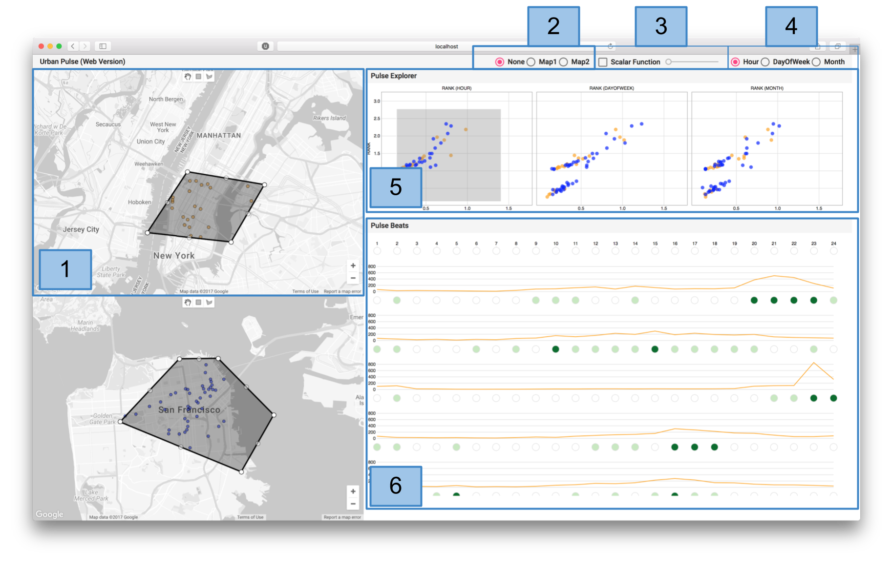
-
The maps on the left show the computed pulses in each city. Pulses can be selected by brushing with one of the selection tools available on the top part of each map. To deselect a brush, right click on top of the brush.
-
The pulse similarity search mode can be activated by choosing
Map1orMap2. -
Enables the display of the scalar function for the temporal resolution selected in 4.
-
Selects a temporal resolution.
-
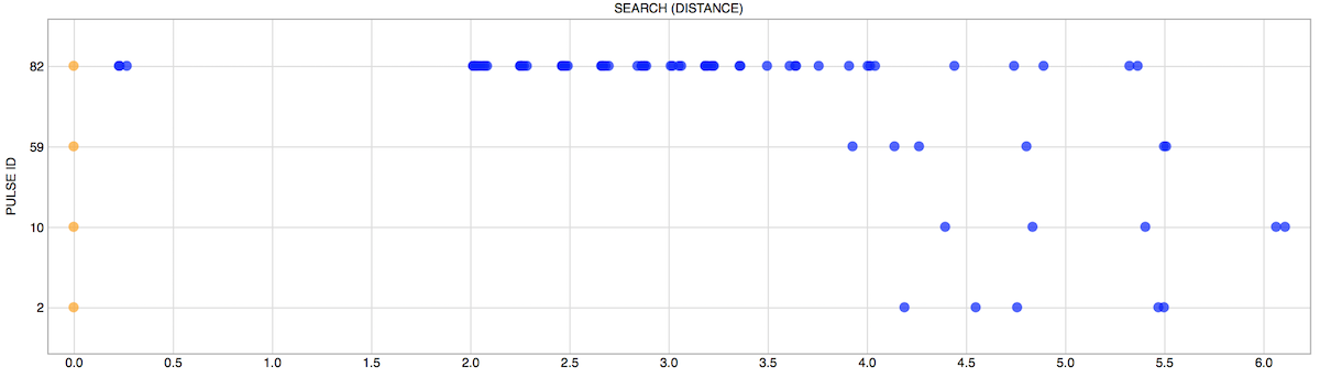
Shows the pulses in three different temporal resolutions. If pulse similarity search mode is selected, displays a single plot with the similarity measures for all selected pulses:
- Shows the beats for all selected pulses. The circles on the top allow for filtering of pulses with certain beat values.
