Tfdiffeq Save
Tensorflow implementation of Ordinary Differential Equation Solvers with full GPU support
Tensorflow Ordinary Differential Equation Solvers

A library built to replicate the TorchDiffEq library built for the Neural Ordinary Differential Equations paper by Chen et al, running entirely on Tensorflow Eager Execution.
All credits for the codebase go to @rtqichen for providing an excellent base to reimplement from.
Similar to the PyTorch codebase, this library provides ordinary differential equation (ODE) solvers implemented in Tensorflow Eager. For usage of ODE solvers in deep learning applications, see Neural Ordinary Differential Equations paper.
Supports Augmented Neural ODE Architectures from the paper Augmented Neural ODEs as well, which has been shown to solve certain problems that Neural ODEs may struggle with.
Support for Universal Differential Equations (for ODE case) from the paper Universal Differential Equations for Scientific Machine Learning. While slow, and restricted to ODEs only, it works well enough on Lotke Voltera system as described in example notebook.
Support for Hypersolvers from the paper Hypersolvers: Toward Fast Continuous-Depth Models. Currently implements the paper implementation of HyperEuler and HyperHuen. The paper Deep Euler method: solving ODEs by approximating the local truncation error of the Euler method proposes nearly the same approach. NOTE: These APIs are subject to change once the paper releases source code.
Now supports Adjoint methods for Dopri5 solver due to PR #3 from @eozd.
As the solvers are implemented in Tensorflow, algorithms in this repository fully support running on the GPU, and are differentiable. Also supports prebuilt ODENet and ConvODENet tf.keras Models that can be used as is or embedded in a larger architecture.
Caveats
There are a few major limitations with this project :
- Speed is almost the same as the PyTorch codebase (+- 2%), if the solver is wrapped inside a
tf.deviceblock. Runge-Kutta solvers require double dtype precision for correct gradient computations. Yet, Tensorflow does not provide a convenient global switch to force all created tensors to double dtype. So explicit casts are unavoidable.- Make sure to wrap the entire script in a
with tf.device('/gpu:0')to make full utilization of the GPU. Or select the main components - the model, the optimizer, the dataset and theodeintcall inside tf.device blocks locally. - Convenience method
move_to_deviceis made available from the library to make things easier on this front. - If type errors are thrown, correct them with
tf.cast()
- Make sure to wrap the entire script in a
Notebooks to get started
- There exists a Jupyter Notebook in the examples folder,
ode_usage.ipynbwhich has examples of several ODE solutions, explaining various methods and demonstrates visualization functions available in this library. The Notebook can also be visualized on Google Colab : Colaboratory Link
- An example of Augmented Neural ODEs and Prebuilt ODENet models is available on Google Colab : Colaboratory Link
- An example of Universal Differential Equations for the Lotka-Volterra system is available on Google Colab : Colaboratory Link
Basic Usage
Note: This is taken directly from the original PyTorch codebase. Almost all concepts apply here as well.
This library provides one main interface odeint which contains general-purpose algorithms for solving initial value problems (IVP), with gradients implemented for all main arguments. An initial value problem consists of an ODE and an initial value,
dy/dt = f(t, y) y(t_0) = y_0.
The goal of an ODE solver is to find a continuous trajectory satisfying the ODE that passes through the initial condition.
To solve an IVP using the default solver:
from tfdiffeq import odeint

odeint(func, y0, t)
where func is any callable implementing the ordinary differential equation f(t, x), y0 is an any-D Tensor or a tuple of any-D Tensors representing the initial values, and t is a 1-D Tensor containing the evaluation points. The initial time is taken to be t[0].
Backpropagation through odeint goes through the internals of the solver, but this is not supported for all solvers. Instead, we encourage the use of the adjoint method explained in Neural Ordinary Differential Equations paper, which will allow solving with as many steps as necessary due to O(1) memory usage.
Example of an ODE Model
import tensorflow as tf

class LotkaVolterra(tf.keras.Model):

  def __init__(self, a, b, c, d,):
    super().__init__()
    self.a, self.b, self.c, self.d = a, b, c, d

  @tf.function
  def call(self, t, y):
    # y = [R, F]
    r, f = tf.unstack(y)

    dR_dT = self.a * r - self.b * r * f
    dF_dT = -self.c * f + self.d * r * f

    return tf.stack([dR_dT, dF_dT])
Examples of using Hypersolvers
Please refer to the Colab Notebook - hyper_solvers, in order to see a demonstration of a HyperHuen network trained to evaluate Lorenz Attractor chaotic ODE.
This above notebook includes code blocks to be used as reference to train and evaluate such Hypersolvers.
import tensorflow as tf
from tfdiffeq.hyper import HyperHeun

# Create a Hyper network that HyperHuen will use as the Solver network `g`

class HyperSolverModule(tf.keras.Model):
  def __init__(self, func_input_dim, hidden_dim=64):
    super().__init__(dtype='float64')
    self.func_input_dim = func_input_dim

    # Input dim isnt used (Keras handled it automatically)
    # But for illustration purposes, it is provided
    # Computed as ~ dim(y) + dim(dy) + 1 (for time axis)
    self.input_dim = 2 * func_input_dim + 1
    self.hidden_dim = hidden_dim
    self.output_dim = func_input_dim

    self.g = tf.keras.Sequential([
        tf.keras.layers.Dense(self.hidden_dim),
        tf.keras.layers.PReLU(),
        tf.keras.layers.Dense(self.hidden_dim),
        tf.keras.layers.PReLU(),
        tf.keras.layers.Dense(self.hidden_dim),
        tf.keras.layers.PReLU(),
        tf.keras.layers.Dense(self.output_dim)
    ])

  @tf.function
  def call(self, x):
    return self.g(x)

# Assume we use Lorenz Attractor as the ODE we want to model - `f`

f = Lorenz(sigma, beta, rho)
g = HyperSolverModule(func_input_dim=3, hidden_dim=64)

hyper_heun = HyperHeun(f, g)

# The stepe to train this model are available in the notebook mentioned above
Prebuilt Models
This library now supports prebuilt models inside the tfdiffeq.models namespace - specifically the Neural ODENet and Convolutional Neural ODENet. In addition, both of these models inherently support Augmented Neural ODENets.
They can be used a models themselves, or can be inserted inside a larger stack of ODENet layers to build a deeper ODENet or ConvODENet model, depending on the usecase.
Usage :
import tensorflow as tf
from tfdiffeq.models import ODENet, ConvODENet

# Directly usable model
model = ODENet(hidden_dim, output_dim, augment_dim=0, time_dependent=False)
model = ConvODENet(num_filters, augment_dim=0, time_dependent=False)

# Used inside other models
x = Conv2D(...)(x)
x = Conv2D(...)(x)
x = Flatten()(x)
x = ODENet(...)(x)  # or dont use flatten and use ConvODENet directly
x = ODENet(...)(x)  # or dont use flatten and use ConvODENet directly
...
Keyword Arguments
-
rtol: Relative tolerance. -
atol: Absolute tolerance. -
method: One of the solvers listed below.
List of ODE Solvers:
Adaptive-step:
-
dopri5: Runge-Kutta 4(5) [default]. -
dopri8: Runga-Kutta 8(5). -
adams: Adaptive-order implicit Adams.
Fixed-step:
-
euler: Euler method. -
midpoint: Midpoint method. -
huen: Second-order Runge-Kutta. -
adaptive_heun: Second-order Adaptive Heun method. -
bosh3: Bogacki-Shampine solver (MATLAB ode23). -
rk4: Fourth-order Runge-Kutta with 3/8 rule. -
explicit_adams: Explicit Adams. -
fixed_adams: Implicit Adams
Hyper-solvers (experimental)
-
HyperEuler: Hyper Euler model. -
HyperMidpoint: Hyper Midpoint model. -
HyperHeun: Hyper Heun model.
Compatibility
Since tensorflow doesn't yet support global setting of default datatype, the tfdiffeq library provides a few convenience methods.
-
move_to_device: Attempts to move atf.Tensorto a certain device. Can specify the device in the normal syntax ofcpu:0orgpu:xwherexmust be replaced by any number representing the GPU ID. Falls back to CPU if GPU is unavailable. -
Dont forget to add a
@tf.functionon yourcall(self, t, u)methods defined in a Keras Models for some significant speed up in some cases !
Examples
The scripts for the examples can be found in the examples folder, along with the weights and results for the latent_ode.py script as it takes some time to train. Two results have been replicated from the original codebase:
-
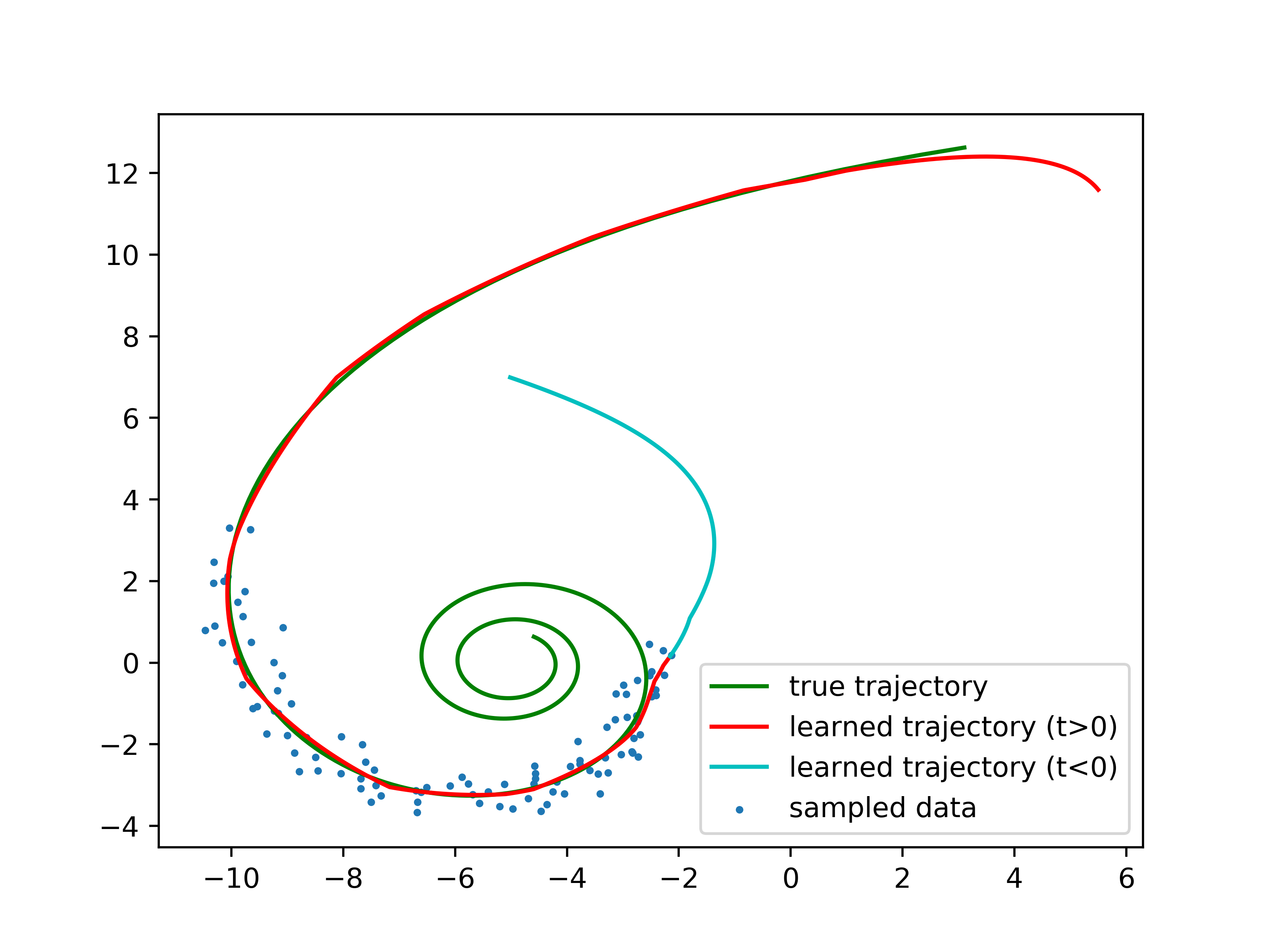
ode_demo.py: A basic example which contains a short implementation of learning a dynamics model to mimic a spiral ODE.
The training should look similar to this:

-
circular_ode_demo.py: A basic example similar to above which contains a short implementation of learning a dynamics model to mimic a circular ODE.
The training should look similar to this:

-
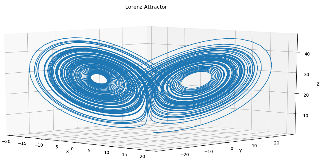
lorenz_attractor.py: A classic example of a chaotic solution for certain parameter sets and initial conditions.
Note this is just a stress test for the library, and scipy.integrate.odefun can solve this much much faster due to highly optimized routines. This should take roughly 1 minute on a modern machine.
-
latent_ode.py: Another basic example which uses variational inference to learn a path along a spiral.
Results should be similar to below after 1200 iterations:
-
ODENeton MNIST
While the Adjoint method is not yet implemented, a smaller version of ODENet can be easily trained using the
fixed grid solvers - Euler or Huens for a fast approximate solution. It has been observed that as MNIST is
an extremely easy problem, RK45 (DOPRI5) works relatively well, whereas on more complex datasets like CIFAR 10/100
it diverges in the first epoch.
Reference : ANODE: Unconditionally Accurate Memory-Efficient Gradients for Neural ODEs

-
Universal Differential Equations
Following the methodology in the paper Universal Differential Equations for Scientific Machine Learning, we reproduce (sub-optimally) the Lotke-Volterra experiment in the following notebook - UniversalNeuralODE.ipynb
References : Universal Differential Equations for Scientific Machine Learning
-
Continious Normalizing Flows
Ported Continious Normalizing Flow example from the torchdiffeq repository - CNF Examples.
References : FFJORD: Free-Form Continuous Dynamics for Scalable Reversible Generative Models

Example of constructing, training and evaluating Hypersolver networks as described in the paper Hypersolvers: Toward Fast Continuous-Depth Models. NOTE: Current API is experiemental and subject to change when the paper releases its code.
References : Hypersolvers: Toward Fast Continuous-Depth Models
Reference
If you found this library useful in your research, please consider citing
@article{chen2018neural,
  title={Neural Ordinary Differential Equations},
  author={Chen, Ricky T. Q. and Rubanova, Yulia and Bettencourt, Jesse and Duvenaud, David},
  journal={Advances in Neural Information Processing Systems},
  year={2018}
}
Requirements
Install the required Tensorflow version along with the package using either
pip install .[tf]  # for cpu
pip install .[tf-gpu]  # for gpu
pip install .[tests]  # for cpu testing
- Tensorflow TF 2 / 1.15.0 or above. Prefereably TF 2.0 when it comes out, as the entire codebase requires Eager Execution.
- Tensorflow Probability (for CNF example only)
- matplotlib
- numpy
- scipy (for tests)
- six
- pysindy (for Universal Differential Equations support only)
