Temporal Ensembling For Semi Supervised Learning Save Abandoned
Implementation of Temporal Ensembling for Semi-Supervised Learning by Laine et al. with tensorflow eager execution
Temporal-Ensembling-for-Semi-Supervised-Learning
This repository includes a implementation of Temportal Ensembling for Semi-Supervised Learning by Laine et al. with Tensorflow eager execution.
When I was reading "Realistic Evaluation of Deep Semi-Supervised Learning Algorithms" by Avital Oliver (2018), I realized I had never played enough with Semi-Supervised Learning, so I came across this paper and thought it was interesting for me to play with. (I highly recommend reading the paper by Avital et al., one of my favorite recent papers). Additionally eager will be the default execution method when the 2.0 Tensorflow version comes out, so I though I should use it in this repository.
Semi-Supervised Learning
Semi-Supervised Learning algorithms try improving traditional supervised learning ones by using unlabeled samples. This is very interesting because in real-world there are a big amount of problems where we have a lot of data that is unlabeled. There is no valid reason why this data cannot be used to learn the general structure of the dataset by supporting the learning process of the supervised training.
Self-Ensembling
The paper propose two implementations of self-ensembling, i.e. forming different ensemble predictions in the training process under different conditions of regularization (dropout) and augmentations.
The two different methods are -Model and temporal ensembling. Let's dive a little bit into each one of them.

Pi Model
In the -Model the training inputs
are evaluated twice, under different conditions of dropout regularization and augmentations, resulting in tow outputs
and
.
The loss function here includes two components:
-
Supervised Component: standard cross-entropy between ground-truth
and predicted values
(only applied to labeled inputs).
-
Unsupervised Component: penalization of different outputs for the same input under different augmentations and dropout conditions by mean square difference minimization between
. This component is applied to all inputs (labeled and unlabeled).
This two components are combined by summing both components and scaling the unsupervised one using a time-dependent weighting function . According to the paper, asking
and
to be close is a much more string requirement than traditional supervised cross-entropy loss.
The augmentations and dropouts are always randomly different for each input resulting in different output predictions. Additionally to the augmentations, the inputs are also combined with random gaussian noise to increase the variability.
The weighting function will be described later since is also used by temporal ensembling, but it ramps up from zero and increases the contribution from the unsupervised component reaching its maximum by 80 epochs. This means that initially the loss and the gradients are mainly dominated by the supervised component (the authors found that this slow ramp-up is important to keep the gradients stable).
One big difficulty of the -Model is that it relies on the output predictions that can be quite unstable during the training process. To combat this instability the authors propose the temporal ensembling.
Temporal Ensembling
Trying to resolve the problem of the noisy predictions during train, temporal ensembling aggregates the predictions of past predictions into an ensemble prediction.
Instead of evaluating each input twice, the predictions are forced to be close the a ensemble prediction
, that is based on previous predictions of the network. This algorithm stores each prediction vector
and in the end of each epoch, these are accumulated in the ensemble vector
by using the formula:
where $\alpha$ is a term that controls how far past predictions influence the temporal ensemble. This vector contains a weighted average of previous predictions for all instances, with recent ones having a higher weight. The ensemble training targets , to be comparable to
need to be scaled by dividing them by
.
In this algorithm, and
are zero on the first epoch, since no past predictions exist.
The advantages of this algorithm when compared to the -Model is:
- Training is approximately 2x faster (only one evaluation per input each epoch)
- The
-Model.
The disadvantages are the following:
- The predictions need to be stored across epochs.
- A new hyperparameter
is introduced.
Training details
To test the two types of ensembling, the authors used a CNN with the following architecture:

The datasets tested were CIFAR-10, CIFAR-100 and SVHN. I will focus on the latter since currently I only tested on this dataset.
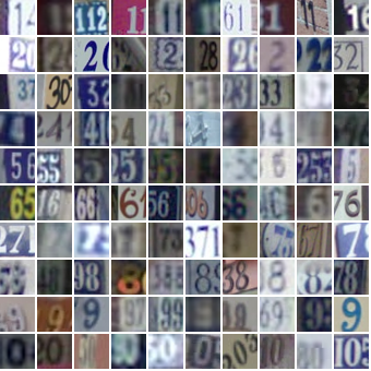
SVHN Dataset
The Street View House Numbers (SVHN) dataset includes images with digits and numbers in natural scene images. The authors used the MNIST-like 32x32 images centered around a single character, trying to classify the center digit. It has 73257 digits for training, 26032 digits for testing, and 531131 extra digits (not used currently).
Unsupervised Weight Function
As described before, both algorithms use a time-dependent weighting function . I the paper the authors use a a Gaussian ramp-up curve that grows from 0 to 1 in 80 epochs, and remains constant for all training:

The function that describes this rampup is: ![rampup]
Notice that the final weight in each epoch corresponds to , where
in the number of labeled samples used, N
is the number of total training samples and
is a constant that varies across the problem and dataset.
The train used Adam, and the learning rate also suffers a rampup in the first 80 epochs and a rampdown in the last 50 epochs (the rampdown is similar to the rampup Gaussian function, but has a scaling constant of 12.5 instead of 5:

The learning rate in each epoch corresponds to the multiplication of this temporal weight function by a max learning rate (hyperparameter) Adam's ![beta1] also was annealed using this function but instead of tending to 0 it converges to 0.5 on the last 50 epochs.
Training parameters
The training hyperparameters described in the paper are different in both algorithms and for the different datasets:
- Weight and mean only batch normalization with momentum of 0.999 was used in all layers.
- The max learning rate was defined as 0.003 except for temporal ensembling in SVHN dataset, where this parameter was set to 0.001.
- the value for
also varied: in pi-model it was set for 100 for SVHN and CIFAR-10 and 300 for CIFAR-100, while for temporal ensembling it was set to 30.
- The training was done for 300 epochs with batch size of 100.
- Data augmentation included random flips (except in SVHN) and random translations with a max translation of +/- 2 pixels.
- In CIFAR datasets ZCA normalization was used and in SVHN zero mean and unit variance normalization was used.
- Adam was used and in SVHN the ![beta2] was set to 0.99 instead of 0.999, since it seemed to avoid gradient explosion.
There are some differences in this repository regarding the paper:
- The authors claim to completely randomize the batches, which means that can be consecutive batches without labeled inputs. The authors said that structured batches can be used to improve the results so I tried to force a fixed fraction of labeled and unlabeled samples per batch.
- The authors tested in CIFAR-10 and CIFAR-100 and with extra support unlabeled dataset for SVHN and CIFAR. Currently the implementation only includes SVHN training.
- Training using with label corruption was tested in the paper, which is not tested in this repository.
- No information is given in the paper on the validation set. In the implementation by default 1000 samples (100 per class) are used as labeled samples, 200 (20 per class) are used for validation. This is way more close to real-world scenarios and was done also in Avital et al. paper "Realistic Evaluation of Deep Semi-Supervised Learning Algorithms." The remaining training set samples are used as unlabeled samples.
- A full epoch is considered when all labeled samples are passed by the network (this means that in one epoch not all unlabeled samples are passed in the network).
Code Details
train_pi_model.py includes the main function for training the -Model on SVHN dataset. You can edit some variables described before in the beginning of the main function. The default parameters are the described in the paper:
# Editable variables
num_labeled_samples = 1000
num_validation_samples = 200
batch_size = 50
epochs = 300
max_learning_rate = 0.001
initial_beta1 = 0.9
final_beta1 = 0.5
checkpoint_directory = './checkpoints/PiModel'
tensorboard_logs_directory = './logs/PiModel'
Similarly, train_temporal_ensembling_model.py includes the main function for training the temporal ensembling model on SVHN:
# Editable variables
num_labeled_samples = 3000
num_validation_samples = 1000
num_train_unlabeled_samples = NUM_TRAIN_SAMPLES - num_labeled_samples - num_validation_samples
batch_size = 150
epochs = 300
max_learning_rate = 0.0002 # 0.001 as recomended in the paper leads to unstable training.
initial_beta1 = 0.9
final_beta1 = 0.5
alpha = 0.6
max_unsupervised_weight = 30 * num_labeled_samples / (NUM_TRAIN_SAMPLES - num_validation_samples)
checkpoint_directory = './checkpoints/TemporalEnsemblingModel'
tensorboard_logs_directory = './logs/TemporalEnsemblingModel'
svnh_loader.py and tfrecord_loader.py have helper classes for downloading the dataset and save them in tfrecords in order to be loaded as tf.data.TFRecordDataset.
pi_model.py is where the model is defined as tf.keras.Model and where some training functions are defined like rampup and rampdown functions, the loss and gradients functions.
In the folder weight_norm_layers there are some edited tensorflow.layers wrappers for allowing weight normalization and mean-only batch normalization in Conv2D and Dense layers as used in the paper.
The code also saves tensorboard logs, plotting loss curves, mean accuracies and the evolution of the unsupervised learning weight and learning rates. In the case of the temporal ensembling the histograms of the temporal ensembling predictions and the normalized training targets are also saved in tensorboard.
Important Notes
- The authors claimed "in SVHN we noticed that optimization tended to explode during the ramp-up period" and I also noticed this. With the incorrect hyperparameters it is possible to lead to non-convergence, especially when you try high maximum learning rates. Most of the times reducing the learning rate solves this problem. In temporal ensembling the learning rate suggested by the author led to this non-convergence (but notice that here batch stratification occurs) so I needed to decrease it. I also noticed that reducing a little bit the ![beta2] value to 0.998 helped in temporal ensembling. This leads me to conclude that the structured batches don't solve the convergence of the algorithms as reported in the paper.
- If you change the parameters of num_labeled_samples and num_validation_samples you need to remove the tfrecords in data folder (otherwise you will reuse the older dataset).
- In the case of temporal ensembling I started to implement without random shuffling to keep track of the temporal ensemble predictions: this made the training process to non-convergence. This was solved by keep tracking of the indexes of the samples in the dataset iterator:
X_labeled_train, y_labeled_train, labeled_indexes = train_labeled_iterator.get_next()
X_unlabeled_train, _, unlabeled_indexes = train_unlabeled_iterator.get_next()
this is only relevant to the temporal ensembling case.
- You can change the epoch number with max ramp-up value changing the second argument of the ramp_up_function
rampup_value = ramp_up_function(epoch, 40)
- Be careful with the batch size. If you maintain the ratio of labeled/unlabeled samples in the batch, a low batch size can lead to non-convergence. Bigger batch sizes or bigger number of labeled samples used lead to a bigger number of labeled samples in each batch, that make the train more stable.
- The results are not exactly the ones reported in the paper with 1000 labels, but I have to admit that I do not have the hardware to find the best parameters with structured batches (the experiments were run in a 860M NVIDIA card).
If you find any bug or have a suggestion feel free to send me an email or create an issue in the repository!
References
- Laine, Samuli, and Timo Aila. "Temporal ensembling for semi-supervised learning." arXiv preprint arXiv:1610.02242 (2016).
- Oliver, Avital, et al. "Realistic Evaluation of Deep Semi-Supervised Learning Algorithms." arXiv preprint arXiv:1804.09170 (2018).
- Salimans, Tim, and Diederik P. Kingma. "Weight normalization: A simple reparameterization to accelerate training of deep neural networks." Advances in Neural Information Processing Systems. 2016.
Credits
I would like to give credit to some repositories that I found while reading the paper that helped me in my implementation.
- Author's Original Implementation in Lasagne
- NVIDIA’s Π Model from “Temporal Ensembling for Semi-Supervised Learning” (ICLR 2017) with TensorFlow.
- John Farret blog post with Pytorch Code on MNIST dataset
- OpenAI original weight norm implementation
- Weight Norm Tensorflow Issue
[rampup]: http://chart.apis.google.com/chart?cht=tx&chl=w(t)=exp(-5(1-(\frac{epoch}{80})^2) [beta1]: http://chart.apis.google.com/chart?cht=tx&chl=\beta_1 [beta2]: http://chart.apis.google.com/chart?cht=tx&chl=\beta_2
