Starcraft2 Replay Analysis Save
A jupyter notebook that provides analysis for StarCraft 2 replays
StarCraft II Replay Analysis with Jupyter Notebooks
In this code pattern we will use Jupyter notebooks to analyze StarCraft II replays and extract interesting insights.
When the reader has completed this code pattern, they will understand how to:
- Create and run a Jupyter notebook in Watson Studio.
- Use Object Storage to access a replay file.
- Use sc2reader to load a replay into a Python object.
- Examine some of the basic replay information in the result.
- Parse the contest details into a usable object.
- Visualize the contest with Bokeh graphics.
- Store the processed replay in Cloudant.
The intended audience for this code pattern is application developers who need to process StarCraft II replay files and build powerful visualizations.

Flow
- The Developer creates a Jupyter notebook from the included starcraft2_replay_analysis.ipynb file
- A Starcraft replay file is loaded into IBM Cloud Object Storage
- The Object is loaded into the Jupyer notebook
- Processed replay is loaded into Cloudant database for storage
Included components
- IBM Watson Studio: Analyze data using RStudio, Jupyter, and Python in a configured, collaborative environment that includes IBM value-adds, such as managed Spark.
- Cloudant NoSQL DB: Cloudant NoSQL DB is a fully managed data layer designed for modern web and mobile applications that leverages a flexible JSON schema.
- IBM Cloud Object Storage: An IBM Cloud service that provides an unstructured cloud data store to build and deliver cost effective apps and services with high reliability and fast speed to market.
Featured technologies
- Jupyter Notebooks: An open-source web application that allows you to create and share documents that contain live code, equations, visualizations and explanatory text.
- sc2reader: A Python library that extracts data from various Starcraft II resources to power tools and services for the SC2 community.
- pandas: A Python library providing high-performance, easy-to-use data structures.
- Bokeh: A Python interactive visualization library.
Watch the Video
Steps
Follow these steps to setup and run this developer code pattern. The steps are described in detail below.
- Clone the repo
- Create a new Watson Studio project
- Create a Cloudant service instance
- Create the notebook in Watson Studio
- Add the replay file
- Add the Cloudant credentials to the notebook
- Run the notebook
- Analyze the results
- Save and share
1. Clone the repo
Clone the starcraft2-replay-analysis repo locally. In a terminal, run:
git clone https://github.com/IBM/starcraft2-replay-analysis
2. Create a new Watson Studio project
-
Log into IBM's Watson Studio. Once in, you'll land on the dashboard.
-
Create a new project by clicking
+ New projectand choosingData Science:
-
Enter a name for the project name and click
Create. -
NOTE: By creating a project in Watson Studio a free tier
Object Storageservice andWatson Machine Learningservice will be created in your IBM Cloud account. Select theFreestorage type to avoid fees.
-
Upon a successful project creation, you are taken to a dashboard view of your project. Take note of the
AssetsandSettingstabs, we'll be using them to associate our project with any external assets (datasets and notebooks) and any IBM cloud services.
3. Create a Cloudant service instance
- Use the menu for
Services > Data Services, then click+ Add serviceandAddandCreatea Cloudant service. - Use the 3-dot actions menu to select
Manage in IBM Cloudfor the new Cloudant service. - Click on
Service credentialsin the left sidebar. - If credentials were not created, click
New credential +to add them. - Use the
View credentialsdropdown and copy the credentials to use in the notebook.
4. Create the notebook in Watson Studio
-
From the new project
Overviewpanel, click+ Add to projecton the top right and choose theNotebookasset type.
-
Fill in the following information:
- Select the
From URLtab. [1] - Enter a
Namefor the notebook and optionally a description. [2] - Under
Notebook URLprovide the following url: https://github.com/IBM/starcraft2-replay-analysis/blob/master/notebooks/starcraft2_replay_analysis.ipynb [3] - For
Runtimeselect thePython 3.5option. [4]

- Select the
-
Click the
Createbutton. -
TIP: Once successfully imported, the notebook should appear in the
Notebookssection of theAssetstab.
5. Add the replay file
Add the replay to the notebook
-
This notebook uses the dataset king_sejong_station_le.sc2replay. We need to load this assets to our project.
-
From the new project
Overviewpanel, click+ Add to projecton the top right and choose theDataasset type.
-
A panel on the right of the screen will appear to assit you in uploading data. Follow the numbered steps in the image below.
- Ensure you're on the
Loadtab. [1] - Click on the
browseoption. From your machine, browse to the location of theking_sejong_station_le.sc2replayfile in this repository, and upload it. [not numbered] - Once uploaded, go to the
Filestab. [2] - Ensure the files appear. [3]

- Ensure you're on the
Create an empty cell for replay code and credentials
Use the + to create an empty cell to hold
the inserted code and credentials. You can put this cell
at the top or anywhere before the Load the replay cell.
Insert to code
After you add the file, use its Insert to code drop-down menu.
Make sure your active cell is the empty one created earlier.
Select Insert StreamingBody object from the drop-down menu.

Note: This cell is marked as a hidden_cell because it contains sensitive credentials.
Fix-up variable names
The inserted code includes a generated method with credentials and then calls
the generated method to set a variable with a name like streaming_body_1. If you do
additional inserts, the method can be re-used and the variable will change
(e.g. streaming_body_2).
Later in the notebook, we set replay_file = streaming_body_1. So you might need to
fix the variable name streaming_body_1 to match your inserted code.
6. Add the Cloudant credentials to the notebook
Use the + button above to create an empty cell to hold the credentials. You can put this cell at the top or anywhere before Storing replay files. You should add a # @hidden_cell line to help you avoid sharing credentials (but be aware that giving people access to the notebook will give them access to your credentials).
Create a variable named credentials_1 (which is used later in the notebook) and paste the Cloudant credentials JSON as the value. The apikey and username will be used. The other credential keys may be included -- they will be ignored.
The code cell should look like this:
# @hidden_cell
credentials_1 = {
  "apikey": "Aa_aAaaa9aAAAa9999A9aa999aaaAaaaAaaA-AAAAA-A",
  "username": "a9999aa9-9aa9-9999-aa99-9a999aaa9a99-bluemix",
  "other": "other credential keys/values are ignored..."
}
7. Run the notebook
When a notebook is executed, what is actually happening is that each code cell in the notebook is executed, in order, from top to bottom.
Each code cell is selectable and is preceded by a tag in the left margin. The tag
format is In [x]:. Depending on the state of the notebook, the x can be:
-
A blank, this indicates that the cell has never been executed.
-
A number, this number represents the relative order this code step was executed.
-
A
*, this indicates that the cell is currently executing. -
Click the
(►) Runbutton to start stepping through the notebook.
8. Analyze the results
The result of running the notebook is a report which may be shared with or without sharing the code. You can share the code for an audience that wants to see how you came your conclusions. The text, code and output/charts are combined in a single web page. For an audience that does not want to see the code, you can share a web page that only shows text and output/charts.
Basic output
Basic replay information is printed out to show you how you can start working with a loaded replay. The output is also, of course, very helpful to identify which replay you are looking at.

Data preparation
If you look through the code, you'll see that a lot of work went into preparing the data.
Unit and building groups
List of strings were created for the known units and groups. These are needed to recognize the event types.
Event handlers
Handler methods were written to process the different types of events and accumulate the information in the player's event list.
The ReplayData class
We created the ReplayData class to take a replay stream of bytes and process
them with all our event handlers. The resulting player event lists are stored
in a ReplayData object. The ReplayData class also has an as_dict()
method. This method returns a Python dictionary that makes it easy to process
the replay events with our Python code. We also use this dict to create a
Cloudant JSON document.
Visualization
To visualize the replay we chose to use 2 different types of charts and show a side-by-side comparison of the competing players.
- Nelson rules charts
- Box plot charts
We generate these charts for each of the following metrics. You will get a good idea of how the players are performing by comparing the trends for these metrics.
- Mineral collection rate
- Vespene collection rate
- Active workers count
- Supply utilization (used / available)
- Worker/supply ratio (workers / supply used)
Box plot charts
Once you get to this point, you can see that generating a box plot is quite easy thanks to pandas DataFrames and Seaborn BoxPlot.
The box plot is a graphical representation of the summary statistics for the metric for each player. The "box" covers the range from the first to the third quartile. The horizontal line in the box shows the mean. The "whisker" shows the spread of data outside these quartiles. Outliers, if any, show up as markers outside the whisker lines. An added swarmplot provides another representation of the distribution of values.
For each metric, we show the players statistics side-by-side using a box plots.

In the above screen shot, you see side-by-side comparison of 4 metrics. In this contest, Neeb had the advantage. In addition to the box which shows the quartiles and the whisker that shows the range, this example has outlier indicators. In many cases, there will be no outliers.
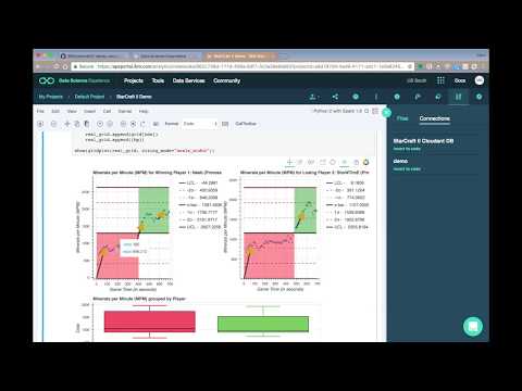
Nelson rules charts
The Nelson rules charts are not so easy. You'll notice quite a bit of code in helper methods to create these charts.
The base chart is a Bokeh plotting figure with circle markers for each data point in the time series. This shows the metric over time for the player. The player charts are side-by-side to allow separate scales and plenty of additional annotations.
We add horizontal lines to show our x-bar (sample mean), 1st and 2nd standard deviations and upper and lower control limits for each player.
We use our detect_nelson_bias() method to detect 9 or more consecutive points
above (or below) the x-bar line. Then, using Bokeh's add_layout() and
BoxAnnotation, we color the background green or red for ranges that show
bias for above or below the line respectively.
Our detect_nelson_trend() method detects when 6 or more consecutive points
are all increasing or decreasing. Using Bokeh's add_layout() and Arrow, we
draw arrows on the chart to highlight these up or down trends.
The result is a side-by-side comparison that is jam-packed with statistical analysis.

In the above screen shot, you see the time/value hover details that you get with Bokeh interactive charts. Also notice the different scales and the arrows. In this contest, Neeb made two early pushes and got an advantage in minerals. If you run the notebook, you'll see other examples showing where the winner got the advantage.
Stored replay documents
You can browse your Cloudant database to see the stored replays. After all the loading and parsing we stored them as JSON documents. You'll see all of your replays in the sc2replays database and only the latest one in sc2recents.
9. Save and share
How to save your work
Under the File menu, there are several ways to save your notebook:
-
Savewill simply save the current state of your notebook, without any version information. -
Save Versionwill save your current state of your notebook with a version tag that contains a date and time stamp. Up to 10 versions of your notebook can be saved, each one retrievable by selecting theRevert To Versionmenu item.
How to share your work
You can share your notebook by selecting the “Share” button located in the top right section of your notebook panel. The end result of this action will be a URL link that will display a “read-only” version of your notebook. You have several options to specify exactly what you want shared from your notebook:
-
Only text and outputwill remove all code cells from the notebook view. -
All content excluding sensitive code cellswill remove any code cells that contain a sensitive tag. For example,# @hidden_cellis used to protect your IBM Cloud credentials from being shared. -
All content, including codedisplays the notebook as is. - A variety of
download asoptions are also available in the menu.
Sample output
The the notebook with output included can be viewed here.
Troubleshooting
License
This code pattern is licensed under the Apache License, Version 2. Separate third-party code objects invoked within this code pattern are licensed by their respective providers pursuant to their own separate licenses. Contributions are subject to the Developer Certificate of Origin, Version 1.1 and the Apache License, Version 2.
