Reinforcement Learning For Decision Making In Self Driving Cars Save
Reinforcement-Learning-for-Decision-Making-in-self-driving-cars
Reinforcement Learning for Decision-Making for self-driving-cars
An practical implementation of RL algorithms for Decision-Making in Autonomous Driving
 |
|---|
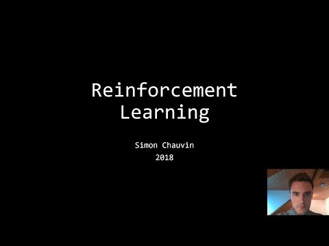
| Related video: Introduction to the concepts of Markov Decision Process (MDP) and Reinforcement Learning (RL) with a focus on the applications for Autonomous Driving |
Structure
My repository is structured as follow. Each time a main, an agent and an environment are required
-
srccontains-
environments- for now, only one simple environment is available
-
main_simple_road.pyis themainfor thesimple_roadenvironment- useful tools for vizualisation help to understand how each agent works
-
brains-
simple_brains.pycontains the definition of simple agents, in particular:- One Monte-Carlo model-free control algorithms
-
q_tableis a collections.defaultdict
-
- Four Temporal-Difference-based model-free control algorithms
-
q_tableis a pandas.DataFrame - Only the
learn()method differs:- Q-learning (= max-SARSA)
- SARSA
- SARSA-lambda
- expected-SARSA
-
- One model-based Dynamic Programming method
-
q_tableis a numpy.array
-
- One Monte-Carlo model-free control algorithms
-
simple_DQN_tensorflow.pycontains the definition of DQN agent with tensorflow- not stable yet
-
simple_DQN_pytorch.pycontains the definition of DQN agent with tensorflow- not stable yet
-
uncomment the
importstatements if you do not want to use it
-
-
Simple_road environment
A very basic scenario, but useful to apply and understand RL concepts.
The envrionment is designed similarly to openai gym env
Use case
Environment definition:
- Mission
- The agent is driving on a straight road, while a pedestrian is standing on the pavement.
- It has to reach the end of the road (the goal) with a certain velocity.
In addition, he must respect different constrains
- apply traffic law
- make sure to drive at a reduce speed when passing close to the pedestrian
Let's make the agent learn how to do that!

To visualize the progress of the driver at each episode, a tkinter-base animation can be used
- The agent is depicted with a square
- The colour of the square represents the velocity of the agent
- The goal is depicted with a circle
("G") - The pedestrians on the side is represented with a black circle
Note1:
- the time between frames can be adjusted in
main_simple_road.py
Note2: to disable the animation:
- to disable the
Tkinterwindow, set inflag_tkinter = Falseinmain_simple_road.py - if you do not want to use
Tkintermodule, set the flag toFalseand uncomment the first line in the definition of theclass Roadinenvironments
Discrete State space:
- the longitudinal position
- the velocity
The initial state is
[0, 3]
Discrete Action space:
-
no_change- Maintain current speed -
speed_up- Accelerate -
speed_up_up- Hard Accelerate -
slow_down- Decelerate -
slow_down_down- Hard Decelerate
Reward Function: classified into 4 groups (See environments road_env.py)
- time efficiency
- traffic law
- safety
- comfort
Transition function:
The transitions are based on the next velocity
- e.g. if the Agent goes for velocity = 3, then its next position will be 3 cells further.
Termination Condition:
- The task is episodic
- One episode terminates after the Agent passed
position = 18 - In order to solve the environment, the agent must get an average return of
+17over100consecutive episodes.- Knowing that the maximum possible return is
18
- Knowing that the maximum possible return is
Finally, hard constrains are used to eliminate certain undesirable behaviours
- it is better to use action-masking rather than penalizing these behaviours in the reward function
- it also increases the learning speed during training by limiting exploration
Dependencies
Create a conda environment:
conda create --name rl-for-ad python=3.6
Install the packages:
pip install -r requirements.txt
Using python 3 with following modules:
- numpy
- matplotlib
- pandas
- random
- time
- json
- pickle - to save the table in .pkl
- tkinter - to run the animation - can be removed with one parameter + 2 line-commentings
- pytorch is required only for the corresponding Deep Q-Network implementation
- tensorflow is required only for the corresponding Deep Q-Network implementation
RL Agents
All the RL algorithms presented in these figures are implemented. Source
 |
|---|
| DP-, MC-, and TD-backups are implemented |
 |
|---|
| Model-based and model-free Control methods are implemented |
Get Started
In src, main_simple_road.py is the central file you want to use.
Choose
-
the control Agent you want to use (uncomment the others)
-
Q-learning(=max-SARSA) -
SARSA -
SARSA-lambda -
expected-SARSA -
Monte-Carlo -
Dynamic Programming
-
-
the task, playing with flags
-
training -
testing -
hyper-parameter tuning
-
-
if you want the environment window to be display
- with the flag
flag_tkinter = Falsefor the simple environment
- with the flag
Results and Analysis:
Q-values
I tried different formats to store the q-values table:
Each one has its advantages and drawbacks.
The q-values are stored in a q-table that looks like:
[id][-------------------------actions---------------------------] [--state features--]
    no_change   speed_up  speed_up_up  slow_down  slow_down_down  position  velocity
0      -4.500  -4.500000       3.1441  -3.434166       -3.177462       0.0       0.0
1      -1.260  -1.260000       9.0490   0.000000        0.000000       2.0       2.0
2       0.396   0.000000       0.0000   0.000000        0.000000       4.0       2.0
3       2.178   0.000000       0.0000   0.000000        0.000000       6.0       2.0
Eligibility Trace for SARSA-Lambda
SARSA-Lambda updates the model by giving reward to all the steps that contribute to the end return. It can consider
- One single step (SARSA) (
lambda=0) - all the steps in the episode (Monte Carlo) (
lambda=1) - in between (
lambda in [0,1])
It is useful to vizualize the Eligibility Trace in the process of SARSA-Lambda. Here is an example of the lambda = 0.2 and gamma = 0.99
The id denotes the index of occurence: the smaller the index, the older the experience.
The first experience has been seem 6 steps ago. Therefore, its trace is 1 * (lambda * gamma) ** 6 = 0.000060.
The trace decay is high due to small value of lambda. For this reason, it is closer to SARSA rather than Monte Carlo.
[id][-------------------------actions---------------------------] [--state features--]
   no_change  speed_up  speed_up_up  slow_down  slow_down_down  position  velocity
0   0.000060  0.000000        0.000        0.0        0.000000       0.0       3.0
1   0.000000  0.000304        0.000        0.0        0.000000       3.0       3.0
2   0.001537  0.000000        0.000        0.0        0.000000       7.0       4.0
3   0.000000  0.000000        0.000        0.0        0.007762      11.0       4.0
4   0.000000  0.000000        0.000        0.0        0.039204      13.0       2.0
5   0.000000  0.000000        0.198        0.0        0.000000      13.0       0.0
6   0.000000  0.000000        1.000        0.0        0.000000      15.0       2.0
7   0.000000  0.000000        0.000        0.0        0.000000      19.0       4.0
Model-Based Control with Dynamic Programming
 |
|---|
| Optimal Policy and Value Function |
The Policy Iteration algorithm approximates the optimal Policy \pi*
Observations:
- the pedestrian is located near
position = 12 - therefore the speed must be smaller than
3when passingposition = 12. Otherwise, an important negative reward is given. - the values of states that are close to
position = 12withvelocity >= 4are therfore very low. There is no chance for these state to slow down enough before passing the pedestrian. Hence, they cannot escape the high penalty.
I noticed that convergence of Policy Iteration is faster (~10 times) than Value Iteration
-
# Duration of Value Iteration = 114.28 - counter = 121 - delta_value_functions = 9.687738053543171e-06 -
# Duration of Policy Iteration = 12.44 - counter = 5 - delta_policy = 0.0 with theta = 1e-3 and final theta = 1e-5 - In addition, on the figure it can be seen that Value Iteration suggests starting with action
no_changewhatever the initial velocity. This cannot be the optimal policy.
Optimal policy
Model-free and Model-based agents all propose trajectories that are close or equal to the optimal one. For instance the following episode (list of "state-action" pairs):
-
[[0, 3], 'no_change', [3, 3], 'no_change', [6, 3], 'no_change', [9, 3], 'slow_down', [11, 2], 'no_change', [13, 2], 'speed_up', [16, 3], 'no_change', [19, 3]]
Which makes sense:
- the agent keeps his initial velocity
- he slows down when approaching the pedestrian
- he then speeds up to reach the goal with the required velocity
Hyper-parameters
It is possible to play with hyper-parameters and appreciate their impacts:
- the traffic parameters (in simple_road_env.py)
- the reward function (in simple_road_env.py)
- the RL-algorithm (in RL_brain.py)
- the hyper-parameters (in RL_brain.py)
 hyper_parameters = (
            method_used,  # the control RL-method
            gamma_learning = 0.99,
            learning_rate_learning = 0.02,
            eps_start_learning = 1.0,
            eps_end_training = 0.02,
            eps_decay_training = 0.998466
        )
Epsilon-decay scheduling
I noticed that the decay rate of the epsilon has a substantial impact on the convergence and the performance of the model-free agents
I implemented an epsilon decay scheduling. At each episode: eps = max(eps_end, eps_decay * eps)
- hence the value
eps_endis reached atepisode_id = log10(eps_end/eps_start) / log10(eps_decay) - in order to reach this plateau in
episode_idepisodes ,eps_decay = (eps_end / eps_start) ** (1/episode_id) - I found that setting
eps_decay_training = 0.998466(i.e. 3000 episodes) helps converging to a robust solution for all model-free agents
Action-masking
I implemented the action_masking mechanism described in Simon Chauvin, "Hierarchical Decision-Making for Autonomous Driving"
It helps reducing exploration and it ensures safety.
This example of q-values for position = 1, when driving at maximal speed = 5, the agent is prevented from speed_up actions (q = -inf).
velocity   no_change  speed_up  speed_up_up  slow_down  slow_down_down
0  -3.444510 -0.892310    -0.493900       -inf            -inf
1   1.107690  1.506100     1.486100  -5.444510            -inf
2   3.506100  3.486100     2.782100  -0.892310       -7.444510
3   5.486100  4.782100         -inf   1.506100       -2.892310
4   6.782100      -inf         -inf   3.486100       -0.493900
5       -inf      -inf         -inf   4.782100        1.486100
Final value coherence checking
In the Bellman equation, if the episode is terminated, then q_target = r (next state has value 0)
- Therefore, in the Optimal Value Function, the q-values of states that are just about to terminate is equal to the reward associated to the transition caused by the action.
- I find it is very useful to monitor of such q-values in the learning process
 |
|---|
| Monitoring of the convergence of a given q-value |
The q-value estimate for the state/action pair ([16, 3], "no_change") converges to the optimal value (+40 = reward[reach end with correct velocity])
Generated files
Overview of the parameters used for the environment
Weights of the Q-table
Plots in the training phase
Plots of the final Q-table
 |
|---|
| Best actions learnt by model-free agent after 4000 episodes |
| Due to the specification of the inital state, the model-free Agent cannot explore all the states. |
 |
|---|
| Returns for each episode, during the training of a model-free agent |
The orange curve shows the average return over 100 consecutive episodes. It reaches the success threshold after 2400 episodes.
Example of settings
After training, env_configuration.json is generated to summarize the configuration.
{
  "min_velocity":0,
  "previous_action":null,
  "initial_state":[
    0,
    3,
    12
  ],
  "max_velocity_2":2,
  "state_ego_velocity":3,
  "obstacle1_coord":[
    12,
    2
  ],
  "actions_list":[
    "no_change",
    "speed_up",
    "speed_up_up",
    "slow_down",
    "slow_down_down"
  ],
  "goal_velocity":3,
  "goal_coord":[
    19,
    1
  ],
  "previous_state_position":0,
  "obstacle":null,
  "initial_position":[
    0,
    0
  ],
  "previous_state_velocity":3,
  "state_features":[
    "position",
    "velocity"
  ],
  "state_obstacle_position":12,
  "obstacle2_coord":[
    1,
    3
  ],
  "rewards_dict":{
    "goal_with_bad_velocity":-40,
    "negative_speed":-15,
    "under_speed":-15,
    "action_change":-2,
    "over_speed":-10,
    "over_speed_near_pedestrian":-40,
    "over_speed_2":-10,
    "per_step_cost":-3,
    "goal_with_good_velocity":40
  },
  "max_velocity_1":4,
  "max_velocity_pedestrian":2,
  "using_tkinter":false,
  "state_ego_position":0,
  "reward":0
}
Future Works
I am working on a more complex environment with a richer state space. Fine-tuning of hyper-parameter for DQN also belongs to the to-do list. Stay tuned!
Acknowledgments
- Initial inspiration from the very good morvanzhou's tutorials
- Project realized while completing the Udacity's Deep Reinforcement Learning Nanodegree program
