Recurrent Neural Network For BitCoin Price Prediction Save
Recurrent Neural Network (LSTM) by using TensorFlow and Keras in Python for BitCoin price prediction
Recurrent-Neural-Network-for-BitCoin-price-prediction
Recurrent Neural Network(LSTM) by using TensorFlow and Keras in Python for BitCoin price prediction
Prerequisites
- Python 3.0+
- ML Lib.(numpy, matplotlib, pandas, scikit learn)
- TensorFlow
- Keras
What are RNNs and why we need that?
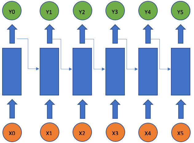
The idea behind RNNs is to make use of sequential information. In a traditional neural network we assume that all inputs (and outputs) are independent of each other. But for many tasks that’s a very bad idea. If you want to predict the next word in a sentence you better know which words came before it. RNNs are called recurrent because they perform the same task for every element of a sequence, with the output being depended on the previous computations. Another way to think about RNNs is that they have a “memory” which captures information about what has been calculated so far. In theory RNNs can make use of information in arbitrarily long sequences, but in practice they are limited to looking back only a few steps (more on this later). Here is what a typical RNN looks like:
Intel Nervana Small Video Introductory Tutorial by Intel Do Check this out
The above diagram shows a RNN being unrolled (or unfolded) into a full network. By unrolling we simply mean that we write out the network for the complete sequence. For example, if the sequence we care about is a sentence of 5 words, the network would be unrolled into a 5-layer neural network.
RNN Extensions
Over the years researchers have developed more sophisticated types of RNNs to deal with some of the shortcomings of the vanilla RNN model.
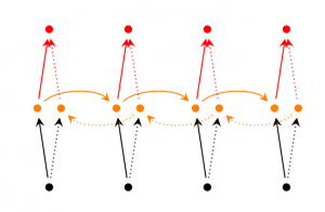
Bidirectional RNN based on the idea that the output at time t may not only depend on the previous elements in the sequence, but also future elements. For example, to predict a missing word in a sequence you want to look at both the left and the right context. Bidirectional RNNs are quite simple. They are just two RNNs stacked on top of each other. The output is then computed based on the hidden state of both RNNs.
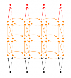
Deep (Bidirectional) RNN similar to Bidirectional RNNs, only that we now have multiple layers per time step. In practice this gives us a higher learning capacity (but we also need a lot of training data).
LSTM Cell
Why LSTM ?
In a traditional recurrent neural network, during the gradient back-propagation phase, the gradient signal can end up being multiplied a large number of times (as many as the number of timesteps) by the weight matrix associated with the connections between the neurons of the recurrent hidden layer. This means that, the magnitude of weights in the transition matrix can have a strong impact on the learning process.
If the weights in this matrix are small (or, more formally, if the leading eigenvalue of the weight matrix is smaller than 1.0), it can lead to a situation called vanishing gradients where the gradient signal gets so small that learning either becomes very slow or stops working altogether. It can also make more difficult the task of learning long-term dependencies in the data. Conversely, if the weights in this matrix are large (or, again, more formally, if the leading eigenvalue of the weight matrix is larger than 1.0), it can lead to a situation where the gradient signal is so large that it can cause learning to diverge. This is often referred to as exploding gradients.
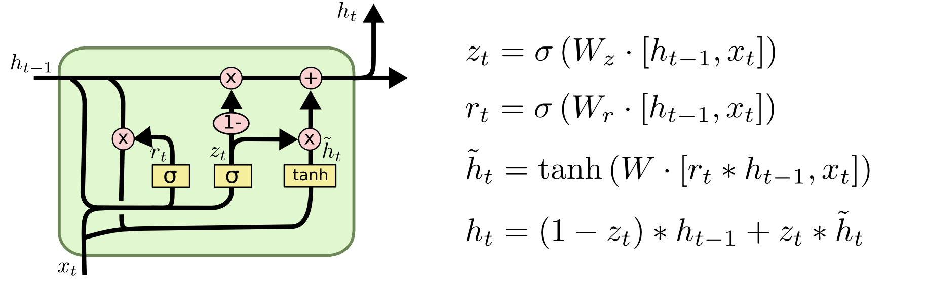
LSTM networks are quite popular these days and we briefly talked about them above. LSTMs don’t have a fundamentally different architecture from RNNs, but they use a different function to compute the hidden state. The memory in LSTMs are called cells and you can think of them as black boxes that take as input the previous state h_{t-1} and current input x_t. Internally these cells decide what to keep in (and what to erase from) memory. They then combine the previous state, the current memory, and the input. It turns out that these types of units are very efficient at capturing long-term dependencies. The repeating module in an LSTM contains four interacting layers.
 LSTM Cell
please do visit for proper explanation [Link]
Implementing LSTM
Importing Data
#Importing the Libraries
import numpy as np
import matplotlib.pyplot as plt
import pandas as pd

#Reading CSV file from train set
training_set = pd.read_csv('Enter the name of file for training_set ')
training_set.head()

#Selecting the second column [for prediction]
training_set = training_set.iloc[:,1:2]
training_set.head()

#Converting into 2D array
training_set = training_set.values
training_set
Scaling
from sklearn.preprocessing import MinMaxScaler
sc = MinMaxScaler()
training_set = sc.fit_transform(training_set)
training_set = sc.fit_transform(training_set)
training_set

X_train = training_set[0:897]
Y_train = training_set[1:898]
Reshaping for keras
#Reshaping for Keras [reshape into 3 dimensions, [batch_size, timesteps, input_dim]
X_train = np.reshape(X_train, (897, 1, 1))
X_train
RNN Layers
from keras.models import Sequential
from keras.layers import Dense
from keras.layers import LSTM
regressor = Sequential()

#Adding the input layer and the LSTM layer
regressor.add(LSTM(units = 4, activation = 'sigmoid', input_shape = (None, 1)))
#Adding the output layer
regressor.add(Dense(units = 1))
#Compiling the Recurrent Neural Network
regressor.compile(optimizer = 'adam', loss = 'mean_squared_error')
#Fitting the Recurrent Neural Network [epoches is a kindoff number of iteration]
regressor.fit(X_train, Y_train, batch_size = 32, epochs = 200)
To prevent Overfitting we can use DropOutLyaer but it's a naive model so it's not really important.
Making Prediction
# Reading CSV file from test set
test_set = pd.read_csv('Enter the name of file for testing_set')
test_set.head()

#selecting the second column from test data
real_btc_price = test_set.iloc[:,1:2]

# Coverting into 2D array
real_btc_price = real_btc_price.values

#getting the predicted BTC value of the first week of Dec 2017
inputs = real_btc_price
inputs = sc.transform(inputs)

#Reshaping for Keras [reshape into 3 dimensions, [batch_size, timesteps, input_dim]
inputs = np.reshape(inputs, (8, 1, 1))
predicted_btc_price = regressor.predict(inputs)
predicted_btc_price = sc.inverse_transform(predicted_btc_price)
Output
#Graphs for predicted values
plt.plot(real_btc_price, color = 'red', label = 'Real BTC Value')
plt.plot(predicted_btc_price, color = 'blue', label = 'Predicted BTC Value')
plt.title('BTC Value Prediction')
plt.xlabel('Days')
plt.ylabel('BTC Value')
plt.legend()
plt.show()

Reference-
Please do visit Great Explanation
- WILDML Tutorial
- StatsBot Blog
- Kimanalytics for Code
