Fendouai Pytorch1.0 Cn Save

PyTorch 1.0 官方文档中文版，欢迎关注微信公众号：磐创AI

Project README

pytorch1.0-cn

pytorch1.0官方文档中文版

PyTorch 入门教程【1】 https://github.com/fendouai/pytorch1.0-cn/blob/master/what-is-pytorch.md

PyTorch 自动微分【2】 https://github.com/fendouai/pytorch1.0-cn/blob/master/autograd-automatic-differentiation.md

PyTorch 神经网络【3】 https://github.com/fendouai/pytorch1.0-cn/blob/master/neural-networks.md

PyTorch 图像分类器【4】 https://github.com/fendouai/pytorch1.0-cn/blob/master/training-a-classifier.md

PyTorch 数据并行处理【5】 https://github.com/fendouai/pytorch1.0-cn/blob/master/optional-data-parallelism.md

PytorchChina:

http://pytorchchina.com

PyTorch 入门教程【1】

什么是 PyTorch?

PyTorch 是一个基于 Python 的科学计算包，主要定位两类人群：

NumPy 的替代品，可以利用 GPU 的性能进行计算。
深度学习研究平台拥有足够的灵活性和速度

开始学习

Tensors (张量)

Tensors 类似于 NumPy 的 ndarrays ，同时 Tensors 可以使用 GPU 进行计算。

from __future__ import print_function
import torch

构造一个5x3矩阵，不初始化。

x = torch.empty(5, 3)
print(x)

输出:

tensor(1.00000e-04 *
       [[-0.0000,  0.0000,  1.5135],
        [ 0.0000,  0.0000,  0.0000],
        [ 0.0000,  0.0000,  0.0000],
        [ 0.0000,  0.0000,  0.0000],
        [ 0.0000,  0.0000,  0.0000]])

构造一个随机初始化的矩阵：

x = torch.rand(5, 3)
print(x)

输出:

tensor([[ 0.6291,  0.2581,  0.6414],
        [ 0.9739,  0.8243,  0.2276],
        [ 0.4184,  0.1815,  0.5131],
        [ 0.5533,  0.5440,  0.0718],
        [ 0.2908,  0.1850,  0.5297]])

构造一个矩阵全为 0，而且数据类型是 long.

Construct a matrix filled zeros and of dtype long:

x = torch.zeros(5, 3, dtype=torch.long)
print(x)

输出:

tensor([[ 0,  0,  0],
        [ 0,  0,  0],
        [ 0,  0,  0],
        [ 0,  0,  0],
        [ 0,  0,  0]])

构造一个张量，直接使用数据：

x = torch.tensor([5.5, 3])
print(x)

输出:

tensor([ 5.5000,  3.0000])

创建一个 tensor 基于已经存在的 tensor。

x = x.new_ones(5, 3, dtype=torch.double)      
# new_* methods take in sizes
print(x)
x = torch.randn_like(x, dtype=torch.float)

# override dtype!
print(x)

# result has the same size

输出:

tensor([[ 1.,  1.,  1.],
        [ 1.,  1.,  1.],
        [ 1.,  1.,  1.],
        [ 1.,  1.,  1.],
        [ 1.,  1.,  1.]], dtype=torch.float64)
tensor([[-0.2183,  0.4477, -0.4053],
        [ 1.7353, -0.0048,  1.2177],
        [-1.1111,  1.0878,  0.9722],
        [-0.7771, -0.2174,  0.0412],
        [-2.1750,  1.3609, -0.3322]])

获取它的维度信息:

print(x.size())

输出:

torch.Size([5, 3])

注意

torch.Size 是一个元组，所以它支持左右的元组操作。

操作

在接下来的例子中，我们将会看到加法操作。

加法: 方式 1

y = torch.rand(5, 3)
print(x + y)

Out:

tensor([[-0.1859,  1.3970,  0.5236],
        [ 2.3854,  0.0707,  2.1970],
        [-0.3587,  1.2359,  1.8951],
        [-0.1189, -0.1376,  0.4647],
        [-1.8968,  2.0164,  0.1092]])

加法: 方式2

print(torch.add(x, y))

Out:

tensor([[-0.1859,  1.3970,  0.5236],
        [ 2.3854,  0.0707,  2.1970],
        [-0.3587,  1.2359,  1.8951],
        [-0.1189, -0.1376,  0.4647],
        [-1.8968,  2.0164,  0.1092]])

加法: 提供一个输出 tensor 作为参数

result = torch.empty(5, 3)
torch.add(x, y, out=result)
print(result)

Out:

tensor([[-0.1859,  1.3970,  0.5236],
        [ 2.3854,  0.0707,  2.1970],
        [-0.3587,  1.2359,  1.8951],
        [-0.1189, -0.1376,  0.4647],
        [-1.8968,  2.0164,  0.1092]])

加法: in-place

# adds x to y
y.add_(x)
print(y)

Out:

tensor([[-0.1859,  1.3970,  0.5236],
        [ 2.3854,  0.0707,  2.1970],
        [-0.3587,  1.2359,  1.8951],
        [-0.1189, -0.1376,  0.4647],
        [-1.8968,  2.0164,  0.1092]])

Note

注意

任何使张量会发生变化的操作都有一个前缀 ''。例如：x.copy(y), x.t_(), 将会改变 x.

你可以使用标准的 NumPy 类似的索引操作

print(x[:, 1])

Out:

tensor([ 0.4477, -0.0048,  1.0878, -0.2174,  1.3609])

改变大小：如果你想改变一个 tensor 的大小或者形状，你可以使用 torch.view:

x = torch.randn(4, 4)
y = x.view(16)
z = x.view(-1, 8)  # the size -1 is inferred from other dimensions
print(x.size(), y.size(), z.size())

Out:

torch.Size([4, 4]) torch.Size([16]) torch.Size([2, 8])

如果你有一个元素 tensor ，使用 .item() 来获得这个 value 。

x = torch.randn(1)
print(x)
print(x.item())

Out:

tensor([ 0.9422])
0.9422121644020081

PyTorch 自动微分【2】

autograd 包是 PyTorch 中所有神经网络的核心。首先让我们简要地介绍它，然后我们将会去训练我们的第一个神经网络。该 autograd 软件包为 Tensors 上的所有操作提供自动微分。它是一个由运行定义的框架，这意味着以代码运行方式定义你的后向传播，并且每次迭代都可以不同。我们从 tensor 和 gradients 来举一些例子。

1、TENSOR

torch.Tensor 是包的核心类。如果将其属性 .requires_grad 设置为 True，则会开始跟踪针对 tensor 的所有操作。完成计算后，您可以调用 .backward() 来自动计算所有梯度。该张量的梯度将累积到 .grad 属性中。

要停止 tensor 历史记录的跟踪，您可以调用 .detach()，它将其与计算历史记录分离，并防止将来的计算被跟踪。

要停止跟踪历史记录（和使用内存），您还可以将代码块使用 with torch.no_grad(): 包装起来。在评估模型时，这是特别有用，因为模型在训练阶段具有 requires_grad = True 的可训练参数有利于调参，但在评估阶段我们不需要梯度。

还有一个类对于 autograd 实现非常重要那就是 Function。Tensor 和 Function 互相连接并构建一个非循环图，它保存整个完整的计算过程的历史信息。每个张量都有一个 .grad_fn 属性保存着创建了张量的 Function 的引用，（如果用户自己创建张量，则g rad_fn 是 None ）。

如果你想计算导数，你可以调用 Tensor.backward()。如果 Tensor 是标量（即它包含一个元素数据），则不需要指定任何参数backward()，但是如果它有更多元素，则需要指定一个gradient 参数来指定张量的形状。

import torch

创建一个张量，设置 requires_grad=True 来跟踪与它相关的计算

x = torch.ones(2, 2, requires_grad=True)
print(x)

输出：

tensor([[1., 1.],
        [1., 1.]], requires_grad=True)

针对张量做一个操作

y = x + 2
print(y)

输出：

tensor([[3., 3.],
        [3., 3.]], grad_fn=)

y 作为操作的结果被创建，所以它有 grad_fn

print(y.grad_fn)

输出：

针对 y 做更多的操作：

z = y * y * 3
out = z.mean()
print(z, out)

输出：

tensor([[27., 27.],
        [27., 27.]], grad_fn=) tensor(27., grad_fn=)

.requires_grad_( ... ) 会改变张量的 requires_grad 标记。输入的标记默认为 False ，如果没有提供相应的参数。

a = torch.randn(2, 2)
a = ((a * 3) / (a - 1))
print(a.requires_grad)
a.requires_grad_(True)
print(a.requires_grad)
b = (a * a).sum()
print(b.grad_fn)

输出：

False
True

梯度：

我们现在后向传播，因为输出包含了一个标量，out.backward() 等同于out.backward(torch.tensor(1.))。

out.backward()

打印梯度 d(out)/dx

print(x.grad)

 输出：

tensor([[4.5000, 4.5000],
        [4.5000, 4.5000]])

原理解释：

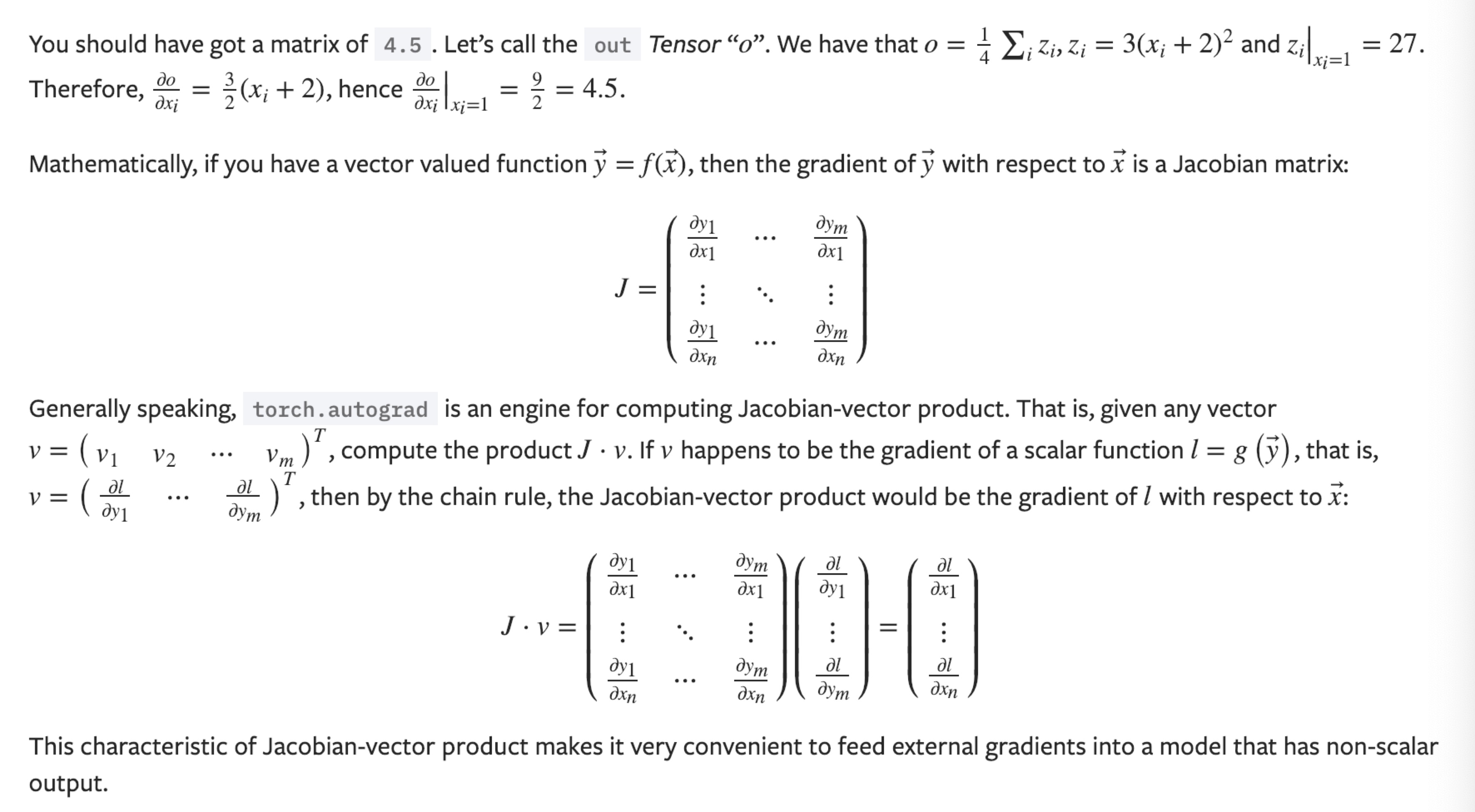
现在让我们看一个雅可比向量积的例子：

x = torch.randn(3, requires_grad=True)
y = x  2
while y.data.norm() < 1000:
y = y  2
print(y)

输出：

tensor([ -444.6791,   762.9810, -1690.0941], grad_fn=)

现在在这种情况下，y 不再是一个标量。torch.autograd 不能够直接计算整个雅可比，但是如果我们只想要雅可比向量积，只需要简单的传递向量给 backward 作为参数。

v = torch.tensor([0.1, 1.0, 0.0001], dtype=torch.float)
y.backward(v)

print(x.grad)

输出：

tensor([1.0240e+02, 1.0240e+03, 1.0240e-01])

你可以通过将代码包裹在 with torch.no_grad()，来停止对从跟踪历史中的 .requires_grad=True 的张量自动求导。

print(x.requires_grad)
print((x ** 2).requires_grad)

with torch.no_grad():
    print((x ** 2).requires_grad)

输出：

True
True
False

稍后可以阅读：

autograd 和 Function 的文档在： https://pytorch.org/docs/autograd

下载 Python 源代码：

autograd_tutorial.py

下载 Jupyter 源代码：

autograd_tutorial.ipynb

PyTorch 神经网络【3】

神经网络

神经网络可以通过 torch.nn 包来构建。

现在对于自动梯度(autograd)有一些了解，神经网络是基于自动梯度 (autograd)来定义一些模型。一个 nn.Module 包括层和一个方法 forward(input) 它会返回输出(output)。

例如，看一下数字图片识别的网络：

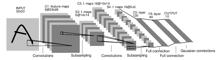
这是一个简单的前馈神经网络，它接收输入，让输入一个接着一个的通过一些层，最后给出输出。

一个典型的神经网络训练过程包括以下几点：

1.定义一个包含可训练参数的神经网络

2.迭代整个输入

3.通过神经网络处理输入

4.计算损失(loss)

5.反向传播梯度到神经网络的参数

6.更新网络的参数，典型的用一个简单的更新方法：weight = weight - learning_rate *gradient

定义神经网络

import torch
import torch.nn as nn
import torch.nn.functional as F


class Net(nn.Module):

    def __init__(self):
        super(Net, self).__init__()
        # 1 input image channel, 6 output channels, 5x5 square convolution
        # kernel
        self.conv1 = nn.Conv2d(1, 6, 5)
        self.conv2 = nn.Conv2d(6, 16, 5)
        # an affine operation: y = Wx + b
        self.fc1 = nn.Linear(16 * 5 * 5, 120)
        self.fc2 = nn.Linear(120, 84)
        self.fc3 = nn.Linear(84, 10)

    def forward(self, x):
        # Max pooling over a (2, 2) window
        x = F.max_pool2d(F.relu(self.conv1(x)), (2, 2))
        # If the size is a square you can only specify a single number
        x = F.max_pool2d(F.relu(self.conv2(x)), 2)
        x = x.view(-1, self.num_flat_features(x))
        x = F.relu(self.fc1(x))
        x = F.relu(self.fc2(x))
        x = self.fc3(x)
        return x

    def num_flat_features(self, x):
        size = x.size()[1:]  # all dimensions except the batch dimension
        num_features = 1
        for s in size:
            num_features *= s
        return num_features


net = Net()
print(net)

输出：

Net(
  (conv1): Conv2d(1, 6, kernel_size=(5, 5), stride=(1, 1))
  (conv2): Conv2d(6, 16, kernel_size=(5, 5), stride=(1, 1))
  (fc1): Linear(in_features=400, out_features=120, bias=True)
  (fc2): Linear(in_features=120, out_features=84, bias=True)
  (fc3): Linear(in_features=84, out_features=10, bias=True)
)

你刚定义了一个前馈函数，然后反向传播函数被自动通过 autograd 定义了。你可以使用任何张量操作在前馈函数上。

一个模型可训练的参数可以通过调用 net.parameters() 返回：

params = list(net.parameters())
print(len(params))
print(params[0].size())  # conv1's .weight

输出：

10
torch.Size([6, 1, 5, 5])

让我们尝试随机生成一个 32x32 的输入。注意：期望的输入维度是 32x32 。为了使用这个网络在 MNIST 数据及上，你需要把数据集中的图片维度修改为 32x32。

input = torch.randn(1, 1, 32, 32)
out = net(input)
print(out)

输出：

tensor([[-0.0233,  0.0159, -0.0249,  0.1413,  0.0663,  0.0297, -0.0940, -0.0135,
          0.1003, -0.0559]], grad_fn=)

把所有参数梯度缓存器置零，用随机的梯度来反向传播

net.zero_grad()
out.backward(torch.randn(1, 10))

在继续之前，让我们复习一下所有见过的类。

torch.Tensor - A multi-dimensional array with support for autograd operations like backward(). Also holds the gradient w.r.t. the tensor. nn.Module - Neural network module. Convenient way of encapsulating parameters, with helpers for moving them to GPU, exporting, loading, etc. nn.Parameter - A kind of Tensor, that is automatically registered as a parameter when assigned as an attribute to a Module. autograd.Function - Implements forward and backward definitions of an autograd operation. Every Tensor operation, creates at least a single Function node, that connects to functions that created a Tensor and encodes its history.

在此，我们完成了：

1.定义一个神经网络

2.处理输入以及调用反向传播

还剩下：

1.计算损失值

2.更新网络中的权重

损失函数

一个损失函数需要一对输入：模型输出和目标，然后计算一个值来评估输出距离目标有多远。

有一些不同的损失函数在 nn 包中。一个简单的损失函数就是 nn.MSELoss ，这计算了均方误差。

例如：

output = net(input)
target = torch.randn(10)  # a dummy target, for example
target = target.view(1, -1)  # make it the same shape as output
criterion = nn.MSELoss()

loss = criterion(output, target)
print(loss)

输出：

tensor(1.3389, grad_fn=)

现在，如果你跟随损失到反向传播路径，可以使用它的 .grad_fn 属性，你将会看到一个这样的计算图：

input -> conv2d -> relu -> maxpool2d -> conv2d -> relu -> maxpool2d
      -> view -> linear -> relu -> linear -> relu -> linear
      -> MSELoss
      -> loss

所以，当我们调用 loss.backward()，整个图都会微分，而且所有的在图中的requires_grad=True 的张量将会让他们的 grad 张量累计梯度。

为了演示，我们将跟随以下步骤来反向传播。

print(loss.grad_fn)  # MSELoss
print(loss.grad_fn.next_functions[0][0])  # Linear
print(loss.grad_fn.next_functions[0][0].next_functions[0][0])  # ReLU

输出：

反向传播

为了实现反向传播损失，我们所有需要做的事情仅仅是使用 loss.backward()。你需要清空现存的梯度，要不然帝都将会和现存的梯度累计到一起。

现在我们调用 loss.backward() ，然后看一下 con1 的偏置项在反向传播之前和之后的变化。

net.zero_grad()     # zeroes the gradient buffers of all parameters

print('conv1.bias.grad before backward')
print(net.conv1.bias.grad)

loss.backward()

print('conv1.bias.grad after backward')
print(net.conv1.bias.grad)

输出：

conv1.bias.grad before backward
tensor([0., 0., 0., 0., 0., 0.])
conv1.bias.grad after backward
tensor([-0.0054,  0.0011,  0.0012,  0.0148, -0.0186,  0.0087])

现在我们看到了，如何使用损失函数。

唯一剩下的事情就是更新神经网络的参数。

更新神经网络参数：

最简单的更新规则就是随机梯度下降。

weight = weight - learning_rate * gradient

我们可以使用 python 来实现这个规则：

learning_rate = 0.01
for f in net.parameters():
    f.data.sub_(f.grad.data * learning_rate)

尽管如此，如果你是用神经网络，你想使用不同的更新规则，类似于 SGD, Nesterov-SGD, Adam, RMSProp, 等。为了让这可行，我们建立了一个小包：torch.optim 实现了所有的方法。使用它非常的简单。

import torch.optim as optim
# create your optimizer
optimizer = optim.SGD(net.parameters(), lr=0.01)
# in your training loop:
optimizer.zero_grad()   # zero the gradient buffers
output = net(input)
loss = criterion(output, target)
loss.backward()
optimizer.step()    # Does the update

下载 Python 源代码：

neural_networks_tutorial.py

下载 Jupyter 源代码：

neural_networks_tutorial.ipynb

PyTorch 图像分类器【4】

你已经了解了如何定义神经网络，计算损失值和网络里权重的更新。

现在你也许会想应该怎么处理数据？

通常来说，当你处理图像，文本，语音或者视频数据时，你可以使用标准 python 包将数据加载成 numpy 数组格式，然后将这个数组转换成 torch.*Tensor

对于图像，可以用 Pillow，OpenCV
对于语音，可以用 scipy，librosa
对于文本，可以直接用 Python 或 Cython 基础数据加载模块，或者用 NLTK 和 SpaCy

特别是对于视觉，我们已经创建了一个叫做 totchvision 的包，该包含有支持加载类似Imagenet，CIFAR10，MNIST 等公共数据集的数据加载模块 torchvision.datasets 和支持加载图像数据数据转换模块 torch.utils.data.DataLoader。

这提供了极大的便利，并且避免了编写“样板代码”。

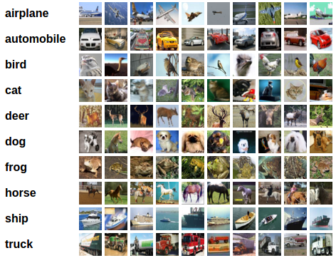
对于本教程，我们将使用CIFAR10数据集，它包含十个类别：‘airplane’, ‘automobile’, ‘bird’, ‘cat’, ‘deer’, ‘dog’, ‘frog’, ‘horse’, ‘ship’, ‘truck’。CIFAR-10 中的图像尺寸为33232，也就是RGB的3层颜色通道，每层通道内的尺寸为32*32。

训练一个图像分类器

我们将按次序的做如下几步：

使用torchvision加载并且归一化CIFAR10的训练和测试数据集
定义一个卷积神经网络
定义一个损失函数
在训练样本数据上训练网络
在测试样本数据上测试网络

加载并归一化 CIFAR10 使用 torchvision ,用它来加载 CIFAR10 数据非常简单。

import torch
import torchvision
import torchvision.transforms as transforms

torchvision 数据集的输出是范围在[0,1]之间的 PILImage，我们将他们转换成归一化范围为[-1,1]之间的张量 Tensors。

transform = transforms.Compose(
    [transforms.ToTensor(),
     transforms.Normalize((0.5, 0.5, 0.5), (0.5, 0.5, 0.5))])
trainset = torchvision.datasets.CIFAR10(root='./data', train=True,
download=True, transform=transform)
trainloader = torch.utils.data.DataLoader(trainset, batch_size=4,
shuffle=True, num_workers=2)
testset = torchvision.datasets.CIFAR10(root='./data', train=False,
download=True, transform=transform)
testloader = torch.utils.data.DataLoader(testset, batch_size=4,
shuffle=False, num_workers=2)
classes = ('plane', 'car', 'bird', 'cat',
'deer', 'dog', 'frog', 'horse', 'ship', 'truck')

输出：

Downloading https://www.cs.toronto.edu/~kriz/cifar-10-python.tar.gz to ./data/cifar-10-python.tar.gz
Files already downloaded and verified

让我们来展示其中的一些训练图片。

import matplotlib.pyplot as plt
import numpy as np

# functions to show an image


def imshow(img):
    img = img / 2 + 0.5     # unnormalize
    npimg = img.numpy()
    plt.imshow(np.transpose(npimg, (1, 2, 0)))
    plt.show()


# get some random training images
dataiter = iter(trainloader)
images, labels = dataiter.next()

# show images
imshow(torchvision.utils.make_grid(images))
# print labels
print(' '.join('%5s' % classes[labels[j]] for j in range(4)))

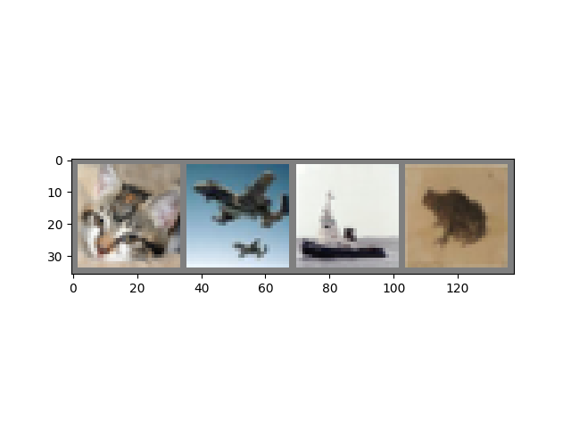
输出：

cat plane  ship  frog

定义一个卷积神经网络在这之前先从神经网络章节复制神经网络，并修改它为3通道的图片(在此之前它被定义为1通道)

import torch.nn as nn
import torch.nn.functional as F
class Net(nn.Module):
def init(self):
super(Net, self).init()
self.conv1 = nn.Conv2d(3, 6, 5)
self.pool = nn.MaxPool2d(2, 2)
self.conv2 = nn.Conv2d(6, 16, 5)
self.fc1 = nn.Linear(16  5  5, 120)
self.fc2 = nn.Linear(120, 84)
self.fc3 = nn.Linear(84, 10)
<span class="k">def</span> <span class="nf">forward</span><span class="p">(</span><span class="bp">self</span><span class="p">,</span> <span class="n">x</span><span class="p">):</span>
    <span class="n">x</span> <span class="o">=</span> <span class="bp">self</span><span class="o">.</span><span class="n">pool</span><span class="p">(</span><span class="n">F</span><span class="o">.</span><span class="n">relu</span><span class="p">(</span><span class="bp">self</span><span class="o">.</span><span class="n">conv1</span><span class="p">(</span><span class="n">x</span><span class="p">)))</span>
    <span class="n">x</span> <span class="o">=</span> <span class="bp">self</span><span class="o">.</span><span class="n">pool</span><span class="p">(</span><span class="n">F</span><span class="o">.</span><span class="n">relu</span><span class="p">(</span><span class="bp">self</span><span class="o">.</span><span class="n">conv2</span><span class="p">(</span><span class="n">x</span><span class="p">)))</span>
    <span class="n">x</span> <span class="o">=</span> <span class="n">x</span><span class="o">.</span><span class="n">view</span><span class="p">(</span><span class="o">-</span><span class="mi">1</span><span class="p">,</span> <span class="mi">16</span> <span class="o">*</span> <span class="mi">5</span> <span class="o">*</span> <span class="mi">5</span><span class="p">)</span>
    <span class="n">x</span> <span class="o">=</span> <span class="n">F</span><span class="o">.</span><span class="n">relu</span><span class="p">(</span><span class="bp">self</span><span class="o">.</span><span class="n">fc1</span><span class="p">(</span><span class="n">x</span><span class="p">))</span>
    <span class="n">x</span> <span class="o">=</span> <span class="n">F</span><span class="o">.</span><span class="n">relu</span><span class="p">(</span><span class="bp">self</span><span class="o">.</span><span class="n">fc2</span><span class="p">(</span><span class="n">x</span><span class="p">))</span>
    <span class="n">x</span> <span class="o">=</span> <span class="bp">self</span><span class="o">.</span><span class="n">fc3</span><span class="p">(</span><span class="n">x</span><span class="p">)</span>
    <span class="k">return</span> <span class="n">x</span>

net = Net()

定义一个损失函数和优化器让我们使用分类交叉熵Cross-Entropy 作损失函数，动量SGD做优化器。

import torch.optim as optim
criterion = nn.CrossEntropyLoss()
optimizer = optim.SGD(net.parameters(), lr=0.001, momentum=0.9)

训练网络这里事情开始变得有趣，我们只需要在数据迭代器上循环传给网络和优化器输入就可以。

for epoch in range(2):  # loop over the dataset multiple times
<span class="n">running_loss</span> <span class="o">=</span> <span class="mf">0.0</span>
<span class="k">for</span> <span class="n">i</span><span class="p">,</span> <span class="n">data</span> <span class="ow">in</span> <span class="nb">enumerate</span><span class="p">(</span><span class="n">trainloader</span><span class="p">,</span> <span class="mi">0</span><span class="p">):</span>
    <span class="c1"># get the inputs</span>
    <span class="n">inputs</span><span class="p">,</span> <span class="n">labels</span> <span class="o">=</span> <span class="n">data</span>

    <span class="c1"># zero the parameter gradients</span>
    <span class="n">optimizer</span><span class="o">.</span><span class="n">zero_grad</span><span class="p">()</span>

    <span class="c1"># forward + backward + optimize</span>
    <span class="n">outputs</span> <span class="o">=</span> <span class="n">net</span><span class="p">(</span><span class="n">inputs</span><span class="p">)</span>
    <span class="n">loss</span> <span class="o">=</span> <span class="n">criterion</span><span class="p">(</span><span class="n">outputs</span><span class="p">,</span> <span class="n">labels</span><span class="p">)</span>
    <span class="n">loss</span><span class="o">.</span><span class="n">backward</span><span class="p">()</span>
    <span class="n">optimizer</span><span class="o">.</span><span class="n">step</span><span class="p">()</span>

    <span class="c1"># print statistics</span>
    <span class="n">running_loss</span> <span class="o">+=</span> <span class="n">loss</span><span class="o">.</span><span class="n">item</span><span class="p">()</span>
    <span class="k">if</span> <span class="n">i</span> <span class="o">%</span> <span class="mi">2000</span> <span class="o">==</span> <span class="mi">1999</span><span class="p">:</span>    <span class="c1"># print every 2000 mini-batches</span>
        <span class="k">print</span><span class="p">(</span><span class="s1">'[</span><span class="si">%d</span><span class="s1">, </span><span class="si">%5d</span><span class="s1">] loss: </span><span class="si">%.3f</span><span class="s1">'</span> <span class="o">%</span>
              <span class="p">(</span><span class="n">epoch</span> <span class="o">+</span> <span class="mi">1</span><span class="p">,</span> <span class="n">i</span> <span class="o">+</span> <span class="mi">1</span><span class="p">,</span> <span class="n">running_loss</span> <span class="o">/</span> <span class="mi">2000</span><span class="p">))</span>
        <span class="n">running_loss</span> <span class="o">=</span> <span class="mf">0.0</span>

print('Finished Training')

 输出：

[1,  2000] loss: 2.187
[1,  4000] loss: 1.852
[1,  6000] loss: 1.672
[1,  8000] loss: 1.566
[1, 10000] loss: 1.490
[1, 12000] loss: 1.461
[2,  2000] loss: 1.389
[2,  4000] loss: 1.364
[2,  6000] loss: 1.343
[2,  8000] loss: 1.318
[2, 10000] loss: 1.282
[2, 12000] loss: 1.286
Finished Training

在测试集上测试网络我们已经通过训练数据集对网络进行了2次训练，但是我们需要检查网络是否已经学到了东西。

我们将用神经网络的输出作为预测的类标来检查网络的预测性能，用样本的真实类标来校对。如果预测是正确的，我们将样本添加到正确预测的列表里。

好的，第一步，让我们从测试集中显示一张图像来熟悉它。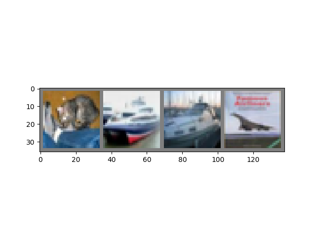

输出：

GroundTruth:    cat  ship  ship plane

现在让我们看看神经网络认为这些样本应该预测成什么：

outputs = net(images)

输出是预测与十个类的近似程度，与某一个类的近似程度越高，网络就越认为图像是属于这一类别。所以让我们打印其中最相似类别类标：

_, predicted = torch.max(outputs, 1)
print('Predicted: ', ' '.join('%5s' % classes[predicted[j]]
for j in range(4)))

输出：

Predicted:    cat  ship   car  ship

结果看起开非常好，让我们看看网络在整个数据集上的表现。

correct = 0
total = 0
with torch.no_grad():
    for data in testloader:
        images, labels = data
        outputs = net(images)
        _, predicted = torch.max(outputs.data, 1)
        total += labels.size(0)
        correct += (predicted == labels).sum().item()
print('Accuracy of the network on the 10000 test images: %d %%' % (
100 * correct / total))

输出：

Accuracy of the network on the 10000 test images: 54 %

这看起来比随机预测要好，随机预测的准确率为10%（随机预测出为10类中的哪一类）。看来网络学到了东西。

class_correct = list(0. for i in range(10))
class_total = list(0. for i in range(10))
with torch.no_grad():
    for data in testloader:
        images, labels = data
        outputs = net(images)
        _, predicted = torch.max(outputs, 1)
        c = (predicted == labels).squeeze()
        for i in range(4):
            label = labels[i]
            class_correct[label] += c[i].item()
            class_total[label] += 1
for i in range(10):
print('Accuracy of %5s : %2d %%' % (
classes[i], 100 * class_correct[i] / class_total[i]))

输出：

Accuracy of plane : 57 %
Accuracy of   car : 73 %
Accuracy of  bird : 49 %
Accuracy of   cat : 54 %
Accuracy of  deer : 18 %
Accuracy of   dog : 20 %
Accuracy of  frog : 58 %
Accuracy of horse : 74 %
Accuracy of  ship : 70 %
Accuracy of truck : 66 %

所以接下来呢？

我们怎么在GPU上跑这些神经网络？

在GPU上训练就像你怎么把一个张量转移到GPU上一样，你要将神经网络转到GPU上。如果CUDA可以用，让我们首先定义下我们的设备为第一个可见的cuda设备。

device = torch.device("cuda:0" if torch.cuda.is_available() else "cpu")

# Assume that we are on a CUDA machine, then this should print a CUDA device:

print(device)

输出：

cuda:0

本节剩余部分都会假定设备就是台CUDA设备。

接着这些方法会递归地遍历所有模块，并将它们的参数和缓冲器转换为CUDA张量。

net.to(device)

记住你也必须在每一个步骤向GPU发送输入和目标：

inputs, labels = inputs.to(device), labels.to(device)

为什么没有注意到与CPU相比巨大的加速？因为你的网络非常小。

练习：尝试增加你的网络宽度（首个 nn.Conv2d 参数设定为 2，第二个nn.Conv2d参数设定为1--它们需要有相同的个数），看看会得到怎么的速度提升。

目标：

深度理解了PyTorch的张量和神经网络
训练了一个小的神经网络来分类图像

在多个GPU上训练

如果你想要来看到大规模加速，使用你的所有GPU，请查看：数据并行性（https://pytorch.org/tutorials/beginner/blitz/data_parallel_tutorial.html）。PyTorch 60 分钟入门教程：数据并行处理

http://pytorchchina.com/2018/12/11/optional-data-parallelism/

下载 Python 源代码：

cifar10_tutorial.py

下载 Jupyter 源代码：

cifar10_tutorial.ipynb

PyTorch 数据并行处理【5】

可选择：数据并行处理（文末有完整代码下载）作者：Sung Kim 和 Jenny Kang

在这个教程中，我们将学习如何用 DataParallel 来使用多 GPU。通过 PyTorch 使用多个 GPU 非常简单。你可以将模型放在一个 GPU：

 device = torch.device("cuda:0")
 model.to(device)

然后，你可以复制所有的张量到 GPU：

 mytensor = my_tensor.to(device)

请注意，只是调用 my_tensor.to(device) 返回一个 my_tensor 新的复制在GPU上，而不是重写 my_tensor。你需要分配给他一个新的张量并且在 GPU 上使用这个张量。

在多 GPU 中执行前馈，后馈操作是非常自然的。尽管如此，PyTorch 默认只会使用一个 GPU。通过使用 DataParallel 让你的模型并行运行，你可以很容易的在多 GPU 上运行你的操作。

 model = nn.DataParallel(model)

这是整个教程的核心，我们接下来将会详细讲解。引用和参数

引入 PyTorch 模块和定义参数

 import torch
 import torch.nn as nn
 from torch.utils.data import Dataset, DataLoader

参数

 input_size = 5
 output_size = 2

 batch_size = 30
 data_size = 100

设备

device = torch.device("cuda:0" if torch.cuda.is_available() else "cpu")

实验（玩具）数据

生成一个玩具数据。你只需要实现 getitem.

class RandomDataset(Dataset):

    def __init__(self, size, length):
        self.len = length
        self.data = torch.randn(length, size)

    def __getitem__(self, index):
        return self.data[index]

    def __len__(self):
        return self.len

rand_loader = DataLoader(dataset=RandomDataset(input_size, data_size),batch_size=batch_size, shuffle=True)

简单模型

为了做一个小 demo，我们的模型只是获得一个输入，执行一个线性操作，然后给一个输出。尽管如此，你可以使用 DataParallel 在任何模型(CNN, RNN, Capsule Net 等等.)

我们放置了一个输出声明在模型中来检测输出和输入张量的大小。请注意在 batch rank 0 中的输出。

class Model(nn.Module):
    # Our model

    def __init__(self, input_size, output_size):
        super(Model, self).__init__()
        self.fc = nn.Linear(input_size, output_size)

    def forward(self, input):
        output = self.fc(input)
        print("\tIn Model: input size", input.size(),
              "output size", output.size())

        return output

创建模型并且数据并行处理

这是整个教程的核心。首先我们需要一个模型的实例，然后验证我们是否有多个 GPU。如果我们有多个 GPU，我们可以用 nn.DataParallel 来包裹我们的模型。然后我们使用 model.to(device) 把模型放到多 GPU 中。

model = Model(input_size, output_size)
if torch.cuda.device_count() > 1:
  print("Let's use", torch.cuda.device_count(), "GPUs!")
  # dim = 0 [30, xxx] -> [10, ...], [10, ...], [10, ...] on 3 GPUs
  model = nn.DataParallel(model)

model.to(device)

输出：

Let's use 2 GPUs!

运行模型：

现在我们可以看到输入和输出张量的大小了。

for data in rand_loader:
    input = data.to(device)
    output = model(input)
    print("Outside: input size", input.size(),
          "output_size", output.size())

输出：

In Model: input size torch.Size([15, 5]) output size torch.Size([15, 2])
        In Model: input size torch.Size([15, 5]) output size torch.Size([15, 2])
Outside: input size torch.Size([30, 5]) output_size torch.Size([30, 2])
        In Model: input size torch.Size([15, 5]) output size torch.Size([15, 2])
        In Model: input size torch.Size([15, 5]) output size torch.Size([15, 2])
Outside: input size torch.Size([30, 5]) output_size torch.Size([30, 2])
        In Model: input size torch.Size([15, 5]) output size torch.Size([15, 2])
        In Model: input size torch.Size([15, 5]) output size torch.Size([15, 2])
Outside: input size torch.Size([30, 5]) output_size torch.Size([30, 2])
        In Model: input size torch.Size([5, 5]) output size torch.Size([5, 2])
        In Model: input size torch.Size([5, 5]) output size torch.Size([5, 2])
Outside: input size torch.Size([10, 5]) output_size torch.Size([10, 2])

结果：

如果你没有 GPU 或者只有一个 GPU，当我们获取 30 个输入和 30 个输出，模型将期望获得 30 个输入和 30 个输出。但是如果你有多个 GPU ，你会获得这样的结果。

多 GPU

如果你有 2 个GPU，你会看到：

# on 2 GPUs
Let's use 2 GPUs!
    In Model: input size torch.Size([15, 5]) output size torch.Size([15, 2])
    In Model: input size torch.Size([15, 5]) output size torch.Size([15, 2])
Outside: input size torch.Size([30, 5]) output_size torch.Size([30, 2])
    In Model: input size torch.Size([15, 5]) output size torch.Size([15, 2])
    In Model: input size torch.Size([15, 5]) output size torch.Size([15, 2])
Outside: input size torch.Size([30, 5]) output_size torch.Size([30, 2])
    In Model: input size torch.Size([15, 5]) output size torch.Size([15, 2])
    In Model: input size torch.Size([15, 5]) output size torch.Size([15, 2])
Outside: input size torch.Size([30, 5]) output_size torch.Size([30, 2])
    In Model: input size torch.Size([5, 5]) output size torch.Size([5, 2])
    In Model: input size torch.Size([5, 5]) output size torch.Size([5, 2])
Outside: input size torch.Size([10, 5]) output_size torch.Size([10, 2])

如果你有 3个GPU，你会看到：

Let's use 3 GPUs!
    In Model: input size torch.Size([10, 5]) output size torch.Size([10, 2])
    In Model: input size torch.Size([10, 5]) output size torch.Size([10, 2])
    In Model: input size torch.Size([10, 5]) output size torch.Size([10, 2])
Outside: input size torch.Size([30, 5]) output_size torch.Size([30, 2])
    In Model: input size torch.Size([10, 5]) output size torch.Size([10, 2])
    In Model: input size torch.Size([10, 5]) output size torch.Size([10, 2])
    In Model: input size torch.Size([10, 5]) output size torch.Size([10, 2])
Outside: input size torch.Size([30, 5]) output_size torch.Size([30, 2])
    In Model: input size torch.Size([10, 5]) output size torch.Size([10, 2])
    In Model: input size torch.Size([10, 5]) output size torch.Size([10, 2])
    In Model: input size torch.Size([10, 5]) output size torch.Size([10, 2])
Outside: input size torch.Size([30, 5]) output_size torch.Size([30, 2])
    In Model: input size torch.Size([4, 5]) output size torch.Size([4, 2])
    In Model: input size torch.Size([4, 5]) output size torch.Size([4, 2])
    In Model: input size torch.Size([2, 5]) output size torch.Size([2, 2])
Outside: input size torch.Size([10, 5]) output_size torch.Size([10, 2])

如果你有 8个GPU，你会看到：

Let's use 8 GPUs!
    In Model: input size torch.Size([4, 5]) output size torch.Size([4, 2])
    In Model: input size torch.Size([4, 5]) output size torch.Size([4, 2])
    In Model: input size torch.Size([2, 5]) output size torch.Size([2, 2])
    In Model: input size torch.Size([4, 5]) output size torch.Size([4, 2])
    In Model: input size torch.Size([4, 5]) output size torch.Size([4, 2])
    In Model: input size torch.Size([4, 5]) output size torch.Size([4, 2])
    In Model: input size torch.Size([4, 5]) output size torch.Size([4, 2])
    In Model: input size torch.Size([4, 5]) output size torch.Size([4, 2])
Outside: input size torch.Size([30, 5]) output_size torch.Size([30, 2])
    In Model: input size torch.Size([4, 5]) output size torch.Size([4, 2])
    In Model: input size torch.Size([4, 5]) output size torch.Size([4, 2])
    In Model: input size torch.Size([4, 5]) output size torch.Size([4, 2])
    In Model: input size torch.Size([4, 5]) output size torch.Size([4, 2])
    In Model: input size torch.Size([4, 5]) output size torch.Size([4, 2])
    In Model: input size torch.Size([4, 5]) output size torch.Size([4, 2])
    In Model: input size torch.Size([2, 5]) output size torch.Size([2, 2])
    In Model: input size torch.Size([4, 5]) output size torch.Size([4, 2])
Outside: input size torch.Size([30, 5]) output_size torch.Size([30, 2])
    In Model: input size torch.Size([4, 5]) output size torch.Size([4, 2])
    In Model: input size torch.Size([4, 5]) output size torch.Size([4, 2])
    In Model: input size torch.Size([4, 5]) output size torch.Size([4, 2])
    In Model: input size torch.Size([4, 5]) output size torch.Size([4, 2])
    In Model: input size torch.Size([4, 5]) output size torch.Size([4, 2])
    In Model: input size torch.Size([4, 5]) output size torch.Size([4, 2])
    In Model: input size torch.Size([4, 5]) output size torch.Size([4, 2])
    In Model: input size torch.Size([2, 5]) output size torch.Size([2, 2])
Outside: input size torch.Size([30, 5]) output_size torch.Size([30, 2])
    In Model: input size torch.Size([2, 5]) output size torch.Size([2, 2])
    In Model: input size torch.Size([2, 5]) output size torch.Size([2, 2])
    In Model: input size torch.Size([2, 5]) output size torch.Size([2, 2])
    In Model: input size torch.Size([2, 5]) output size torch.Size([2, 2])
    In Model: input size torch.Size([2, 5]) output size torch.Size([2, 2])
Outside: input size torch.Size([10, 5]) output_size torch.Size([10, 2])

总结

数据并行自动拆分了你的数据并且将任务单发送到多个 GPU 上。当每一个模型都完成自己的任务之后，DataParallel 收集并且合并这些结果，然后再返回给你。

下载 Python 版本完整代码：

data_parallel_tutorial.py

下载 jupyter notebook 版本完整代码：

data_parallel_tutorial.ipynb

加入 PyTorch 交流 QQ 群：

PytorchChina:

http://pytorchchina.com

Open Source Agenda is not affiliated with "Fendouai Pytorch1.0 Cn" Project. README Source: fendouai/pytorch1.0-cn

Stars

335

Open Issues

Last Commit

5 years ago

Repository

fendouai/pytorch1.0-cn

License

MIT

Homepage

http://pytorchchina.com

Open Source Agenda Badge

<a href="https://www.opensourceagenda.com/projects/pytorch10-cn"><img src="https://www.opensourceagenda.com/projects/pytorch10-cn/reviews/badge.svg" alt="Open Source Agenda"></a>

Submit Review Review Your Favorite Project

Submit Resource Articles, Courses, Videos

Submit Article Submit a post to our blog