OMEinsum - One More Einsum

This is a repository for the Google Summer of Code project on Differentiable Tensor Networks. It implements one function that both computer scientists and physicists love, the Einstein summation

To find out the details about einsum, please check out my nextjournal-article or the numpy-manual.

Einstein summation can be implemented in no more than 20 lines of Julia code, the automatic differentiation is also straightforward. The main effort of this package is improving the performance utilizing Julia multiple dispatch on traits. So that people can enjoy the speed of faster specific implementations like BLAS functions, sum and permutedims on both CPU and GPU without suffering from runtime overhead.

Note: why the test coverage is not 100% - GPU-code coverage is not evaluated although we test the GPU code properly on gitlab. Ignoring the GPU-code, the actual coverage is at about 97%.

Warning: since v0.4, OMEinsum does not optimize the contraction order anymore. One has to use nested einsum to specify the contraction order manually, e.g. ein"(ijk,jkl),klm->im"(x, y, z).

Install

To install, type ] in a julia (>=1.5) REPL and then input

pkg> add OMEinsum

Learn by Examples

To avoid runtime overhead, we recommend users to use non-standard string literal @ein_str. The following examples illustrates how einsum works

julia> using OMEinsum, SymEngine

julia> catty = fill(Basic(:🐱), 2, 2)
2×2 Array{Basic,2}:
 🐱  🐱
 🐱  🐱

julia> fish = fill(Basic(:🐟), 2, 3, 2)
2×3×2 Array{Basic,3}:
[:, :, 1] =
 🐟  🐟  🐟
 🐟  🐟  🐟

[:, :, 2] =
 🐟  🐟  🐟
 🐟  🐟  🐟

julia> snake = fill(Basic(:🐍), 3, 3)
3×3 Array{Basic,2}:
 🐍  🐍  🐍
 🐍  🐍  🐍
 🐍  🐍  🐍

julia> medicine = ein"ij,jki,kk->k"(catty, fish, snake)
3-element Array{Basic,1}:
 4*🐱*🐍*🐟
 4*🐱*🐍*🐟
 4*🐱*🐍*🐟

julia> ein"ik,kj -> ij"(catty, catty) # multiply two matrices `a` and `b`
2×2 Array{Basic,2}:
 2*🐱^2  2*🐱^2
 2*🐱^2  2*🐱^2

julia> ein"ij -> "(catty)[] # sum a matrix, output 0-dimensional array
4*🐱

julia> ein"->ii"(asarray(snake[1,1]), size_info=Dict('i'=>5)) # get 5 x 5 identity matrix
5×5 Array{Basic,2}:
 🐍  0  0  0  0
 0  🐍  0  0  0
 0  0  🐍  0  0
 0  0  0  🐍  0
 0  0  0  0  🐍

Alternatively, people can specify the contraction with a construction approach, which is useful when the contraction code can only be obtained at run time

julia> einsum(EinCode((('i','k'),('k','j')),('i','j')),(a,b))

or a macro based interface, @ein macro, which is closer to the standard way of writing einsum-operations in physics

julia> @ein c[i,j] := a[i,k] * b[k,j];

A table for reference

Many of these are handled by special kernels (listed in the docs), but there is also a fallback which handles other cases (more like what Einsum.jl does, plus a GPU version).

It is sometimes helpful to specify the order of operations, by inserting brackets, either because you know this will be more efficient, or to help the computer see what kernels can be used. For example:

julia> @ein Z[o,s] := x[i,s] * (W[o,i,j] * y[j,s]);   # macro style

julia> Z = ein"is, (oij, js) -> os"(x, W, y);         # string style

This performs matrix multiplication (summing over j) followed by batched matrix multiplication (summing over i, batch label s). Without the brackets, instead it uses the fallback loop_einsum, which is slower. Calling allow_loops(false) will print an error to help you spot such cases:

julia> @ein Zl[o,s] := x[i,s] * W[o,i,j] * y[j,s];

julia> Z ≈ Zl
true

julia> allow_loops(false);

julia> Zl = ein"is, oij, js -> os"(x, W, y);
┌ Error: using `loop_einsum` to evaluate
│   code = is, oij, js -> os
│   size.(xs) = ((10, 50), (20, 10, 10), (10, 50))
│   size(y) = (20, 50)
└ @ OMEinsum ~/.julia/dev/OMEinsum/src/loop_einsum.jl:26

To see more examples using the GPU and autodiff, check out our asciinema-demo here:

Application

For an application in tensor network algorithms, check out the TensorNetworkAD package, where OMEinsum is used to evaluate tensor-contractions, permutations and summations.

Toy Application: solving a 3-coloring problem on the Petersen graph

Let us focus on graphs with vertices with three edges each. A question one might ask is: How many different ways are there to colour the edges of the graph with three different colours such that no vertex has a duplicate colour on its edges?

The counting problem can be transformed into a contraction of rank-3 tensors representing the edges. Consider the tensor s defined as

julia> s = map(x->Int(length(unique(x.I)) == 3), CartesianIndices((3,3,3)))

Then we can simply contract s tensors to get the number of 3 colourings satisfying the above condition! E.g. for two vertices, we get 6 distinct colourings:

julia> ein"ijk,ijk->"(s,s)[]
6

Using that method, it's easy to find that e.g. the peterson graph allows no 3 colouring, since

julia> code = ein"afl,bhn,cjf,dlh,enj,ago,big,cki,dmk,eom->"
afl, bhn, cjf, dlh, enj, ago, big, cki, dmk, eom 

julia> code(fill(s, 10)...)[]
0

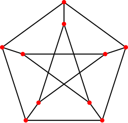
The peterson graph consists of 10 vertices and 15 edges and looks like a pentagram embedded in a pentagon as depicted here:

OMEinsum does not optimie the contraction order by default, so the above contraction can be time consuming. To speed up the contraction, we can use optimize_code to optimize the contraction order:

julia> optcode = optimize_code(code, uniformsize(code, 3), TreeSA())
SlicedEinsum{Char, DynamicNestedEinsum{Char}}(Char[], ago, goa -> 
├─ ago
└─ gcojl, cjal -> goa
   ├─ bgck, bojlk -> gcojl
   │  ├─ big, cki -> bgck
   │  │  ├─ big
   │  │  └─ cki
   │  └─ bhomj, lhmk -> bojlk
   │     ├─ bhn, omnj -> bhomj
   │     │  ├─ bhn
   │     │  └─ eom, enj -> omnj
   │     │     ⋮
   │     │     
   │     └─ dlh, dmk -> lhmk
   │        ├─ dlh
   │        └─ dmk
   └─ cjf, afl -> cjal
      ├─ cjf
      └─ afl
)

julia> contraction_complexity(optcode, uniformsize(optcode, 3))
Time complexity: 2^12.737881076857779
Space complexity: 2^7.92481250360578
Read-write complexity: 2^11.247334178028728

julia> optcode(fill(s, 10)...)[]
0

We can see the time complexity of the optimized code is much smaller than the original one. To know more about the contraction order optimization, please check the julia package OMEinsumContractionOrders.jl.

Confronted with the above result, we can ask whether the peterson graph allows a relaxed variation of 3 colouring, having one vertex that might accept duplicate colours. The answer to that can be found using the gradient w.r.t a vertex:

julia> using Zygote: gradient

julia> gradient(x->optcode(x,s,s,s,s,s,s,s,s,s)[], s)[1] |> sum
0

This tells us that even if we allow duplicates on one vertex, there are no 3-colourings for the peterson graph.

Comparison with other packages

Similar packages include:

• TensorOperations.jl and TensorKit.jl
• ITensors.jl

Comparing with the above packages, OMEinsum is optimized over large scale tensor network (or einsum, sum-product network) contraction. Its main advantages are:

• OMEinsum has better support to very high dimensional tensor networks and their contraction order.
• OMEinsum allows an index to appear multiple times.
• OMEinsum has well tested generic element type support.

However, OMEinsum also has some disadvantages:

• OMEinsum does not support good quantum numbers.
• OMEinsum has less optimization on small scale problems.

Contribute

Suggestions and Comments in the Issues are welcome.

License

MIT License