MINER Pl Save
Unofficial implementation (replicates paper results!) of MINER: Multiscale Implicit Neural Representations in pytorch-lightning
MINER_pl
Unofficial implementation of MINER: Multiscale Implicit Neural Representations in pytorch-lightning.
Official implementation : https://github.com/vishwa91/miner

:open_book: Ref readings
-
My explanatory videos


:warning: Main differences w.r.t. the original paper before continue:
- In the pseudo code on page 8, where the author states Weight sharing for images, it means finer level networks are initialized with coarser level network weights. However, I did not find the correct way to implement this. Therefore, I initialize the network weights from scratch for all levels.
- The paper says it uses sinusoidal activation (does he mean SIREN? I don't know), but I use gaussian activation (in hidden layers) with trainable parameters (per block) like my experiments in the other repo. In finer levels where the model predicts laplacian pyramids, I use sinusoidal activation
x |-> sin(ax)with trainable parametersa(per block) as output layer (btw, this performs significantly better than simpletanh). Moreover, I precompute the maximum amplitude for laplacian residuals, and use it to scale the output, and I find it to be better than without scaling. - I experimented with a common trick in coordinate mlp: positional encoding and find that using it can increase training time/accuracy with the same number of parameters (by reducing 1 layer). This can be turned on/off by specifying the argument
--use_pe. The optimal number of frequencies depends on the patch size, the larger patch sizes, the more number of frequencies you need and vice versa. - Some difference in the hyperparameters: the default learning rate is
3e-2instead of5e-4. Optimizer isRAdaminstead ofAdam. Block pruning happens when the loss is lower than1e-4(i.e. when PSNR>=40) for image and5e-3for occupancy rather than2e-7.
:computer: Installation
- Run
pip install -r requirements.txt. - Download the images from Acknowledgement or prepare your own images into a folder called
images. - Download the meshes from Acknowledgement or prepare your own meshes into a folder called
meshes.
:key: Training
image
Pluto example:
python train.py \
    --task image --path images/pluto.png \
    --input_size 4096 4096 --patch_size 32 32 --batch_size 256 --n_scales 4 \
    --use_pe --n_layers 3 \
    --num_epochs 50 50 50 200 \
    --exp_name pluto4k_4scale
Tokyo station example:
python train.py \
    --task image --path images/tokyo-station.jpg \
    --input_size 6000 4000 --patch_size 25 25 --batch_size 192 --n_scales 5 \
    --use_pe --n_layers 3 \
    --num_epochs 50 50 50 50 150 \
    --exp_name tokyo6k_5scale
| Image (size) | Train time (s) | GPU mem (MiB) | #Params (M) | PSNR |
|---|---|---|---|---|
| Pluto (4096x4096) | 53 | 3171 | 9.16 | 42.14 |
| Pluto (8192x8192) | 106 | 6099 | 28.05 | 45.09 |
| Tokyo station (6000x4000) | 68 | 6819 | 35.4 | 42.48 |
| Shibuya (7168x2560) | 101 | 8967 | 17.73 | 37.78 |
| Shibuya (14336x5120) | 372 | 8847 | 75.42 | 39.32 |
| Shibuya (28672x10240) | 890 | 10255 | 277.37 | 41.93 |
| Shibuya (28672x10240)* | 1244 | 6277 | 98.7 | 37.59 |
*paper settings (6 scales, each network has 4 layer with 9 hidden units)
The original image will be resized to img_wh for reconstruction. You need to make sure img_wh divided by 2^(n_scales-1) (the resolution at the coarsest level) is still a multiple of patch_wh.
mesh
First, convert the mesh to N^3 occupancy grid by
python preprocess_mesh.py --N 512 --M 1 --T 1 --path <path/to/mesh>
This will create N^3 occupancy to be regressed by the neural network.
For detailed options, please see preprocess_mesh.py. Typically, increase M or T if you find the resulting occupancy bad.
Next, start training (bunny example):
python train.py \
    --task mesh --path occupancy/bunny_512.npy \
    --input_size 512 --patch_size 16 --batch_size 512 --n_scales 4 \
    --use_pe --n_freq 5 --n_layers 2 --n_hidden 8 \
    --loss_thr 5e-3 --b_chunks 512 \
    --num_epochs 50 50 50 150 \
    --exp_name bunny512_4scale
For full options, please see here. Some important options:
- If your GPU memory is not enough, try reducing
batch_size. - By default it will not log intermediate images to tensorboard to save time. To visualize image reconstruction and active blocks, add
--log_imageargument.
You are recommended to monitor the training progress by
tensorboard --logdir logs
where you can see training curves and images.
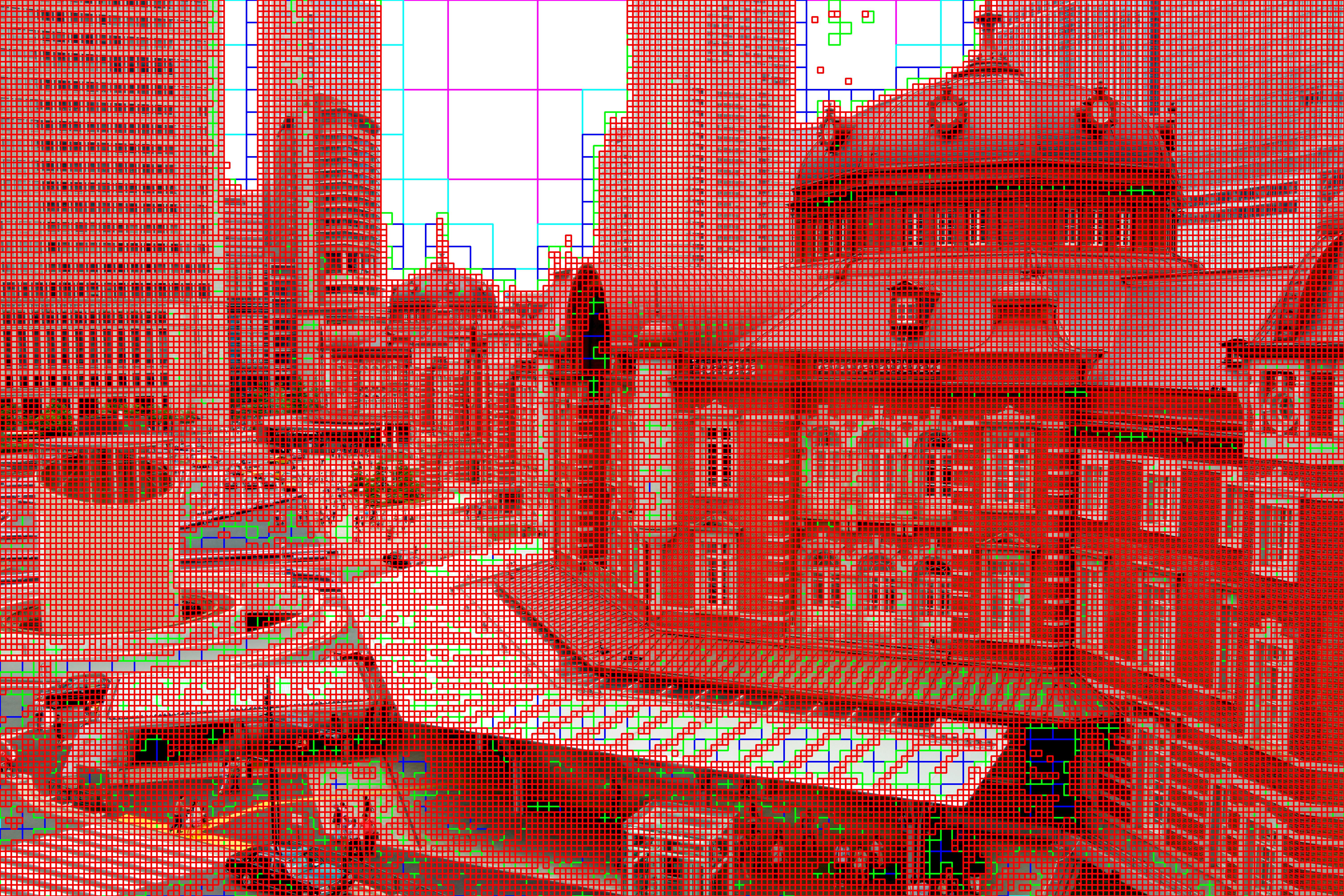
:red_square::green_square::blue_square: Block decomposition
To reconstruct the image using trained model and to visualize block decomposition per scale like Fig. 4 in the paper, see image_test.ipynb or mesh_test.ipynb
Examples:


:bulb: Implementation tricks
- Setting
num_workers=0in dataloader increased the speed a lot. - As suggested in training details on page 4, I implement parallel block inference by defining parameters of shape
(n_blocks, n_in, n_out)and use@operator (same astorch.bmm) for faster inference. - To perform block pruning efficiently, I create two copies of the same network, and continually train and prune one of them while copying the trained parameters to the target network (somehow like in reinforcement learning, e.g. DDPG). This allows the network as well as the optimizer to shrink, therefore achieve higher memory and speed performance.
- In validation, I perform inference in chunks like NeRF, and pass each chunk to cpu to reduce GPU memory usage.
:gift_heart: Acknowledgement
-
Pluto image: NASA
-
Shibuya image: Trevor Dobson
-
Tokyo station image: baroparo
:question: Further readings
During a stream, my audience suggested me to test on this image with random pixels:

The default 32x32 patch size doesn't work well, since the texture varies too quickly inside a patch. Decreasing to 16x16 and increasing network hidden units make the network converge right away to 43.91 dB under a minute. Surprisingly, with the other image reconstruction SOTA instant-ngp, the network is stuck at 17 dB no matter how long I train.

Is this a possible weakness of instant-ngp? What effect could it bring to real application? You are welcome to test other methods to reconstruct this image!
