Imbalanced Ensemble Save
Class-imbalanced Ensemble Learning in Python. | 类别不平衡/长尾机器学习库
![]()
IMBENS: Class-imbalanced Ensemble Learning in Python
![]()
![]()
![]()


![]()


![]()
Documentation: ReadTheDocs | Language: English / 中文
Release:
PyPI |
Source |
Download |
Changelog
Links:
Getting Started |
API Reference |
Examples |
Related Projects |
知乎/Zhihu
Paper:
"IMBENS: Ensemble Class-imbalanced Learning in Python"
IMBENS (imported as imbens) is a Python library for quick implementation, modification, evaluation, and visualization of ensemble learning from class-imbalanced data.
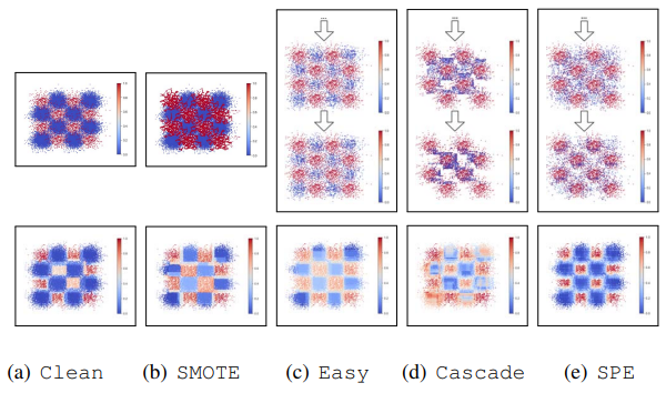
Currently, IMBENS includes over 15 ensemble imbalanced learning algorithms (SMOTEBoost, SMOTEBagging, RUSBoost, EasyEnsemble, BalanceCascade, SelfPacedEnsemble, etc) and also 19 resampling methods (SMOTE, ADASYN, TomekLinks, etc) from imbalance-learn.
IMBENS is featured for:
- 🍎 Unified, easy-to-use APIs with documentation and examples.
- 🍎 Optimized performance with parallelization using joblib.
- 🍎 Powerful, customizable, interactive training logging and visualizer.
- 🍎 Full compatibility with scikit-learn and imbalanced-learn.
- 🍎 Off-the-shelf multi-class imbalanced learning by extending existing techniques.
IMBENS for class-imbalanced classification with <5 lines of code:
# Train an SPE classifier
from imbens.ensemble import SelfPacedEnsembleClassifier
clf = SelfPacedEnsembleClassifier(random_state=42)
clf.fit(X_train, y_train)

# Predict with an SPE classifier
y_pred = clf.predict(X_test)
Citing IMBENS
The IMBENS paper is available on arxiv. If you use IMBENS in a scientific publication, we would appreciate citations to the following paper:
@article{liu2023imbens,
  title={IMBENS: Ensemble Class-imbalanced Learning in Python},
  author={Liu, Zhining and Kang, Jian and Tong, Hanghang and Chang, Yi},
  journal={arXiv preprint arXiv:2111.12776},
  year={2023}
}
Contributing to IMBENS
Please refer to the contributing guidelines.
Table of Contents
- Table of Contents
- Installation
- Highlights
- List of implemented methods
- 5-min Quick Start with IMBENS
- About imbalanced learning
- Acknowledgements
- References
- Related Projects
- Contributors ✨
Installation
It is recommended to use pip for installation.
Please make sure the latest version is installed to avoid potential problems:
$ pip install imbalanced-ensemble            # normal install
$ pip install --upgrade imbalanced-ensemble  # update if needed
Or you can install imbalanced-ensemble by clone this repository:
$ git clone https://github.com/ZhiningLiu1998/imbalanced-ensemble.git
$ cd imbalanced-ensemble
$ pip install .
imbalanced-ensemble requires following dependencies:
- Python (>=3.6)
- numpy (>=1.16.0)
- pandas (>=1.1.3)
- scipy (>=1.9.1)
- joblib (>=0.11)
- scikit-learn (>=1.2.0)
- matplotlib (>=3.3.2)
- seaborn (>=0.11.0)
- tqdm (>=4.50.2)
Highlights
- 🍎 Unified, easy-to-use API design.
All ensemble learning methods implemented in IMBENS share a unified API design. Similar to sklearn, all methods have functions (e.g.,fit(),predict(),predict_proba()) that allow users to deploy them with only a few lines of code. - 🍎 Extended functionalities, wider application scenarios.
All methods in IMBENS are ready for multi-class imbalanced classification. We extend binary ensemble imbalanced learning methods to get them to work under the multi-class scenario. Additionally, for supported methods, we provide more training options like class-wise resampling control, balancing scheduler during the ensemble training process, etc. - 🍎 Detailed training log, quick intuitive visualization.
We provide additional parameters (e.g.,eval_datasets,eval_metrics,training_verbose) infit()for users to control the information they want to monitor during the ensemble training. We also implement anEnsembleVisualizerto quickly visualize the ensemble estimator(s) for providing further information/conducting comparison. See an example here. - 🍎 Wide compatiblilty.
IMBENS is designed to be compatible with scikit-learn (sklearn) and also other compatible projects like imbalanced-learn. Therefore, users can take advantage of various utilities from the sklearn community for data processing/cross-validation/hyper-parameter tuning, etc.
List of implemented methods
Currently (v0.1.3, 2021/06), 16 ensemble imbalanced learning methods were implemented:
(Click to jump to the document page)
-
Resampling-based
- Under-sampling + Ensemble
- Over-sampling + Ensemble
-
Reweighting-based
-
Cost-sensitive Learning
-
AdaCostClassifier[8] -
AdaUBoostClassifier[9] -
AsymBoostClassifier[10]
-
-
Cost-sensitive Learning
- Compatible
Note:
imbalanced-ensembleis still under development, please see API reference for the latest list.
5-min Quick Start with IMBENS
Here, we provide some quick guides to help you get started with IMBENS.
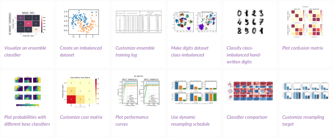
We strongly encourage users to check out the example gallery for more comprehensive usage examples, which demonstrate many advanced features of IMBENS.
A minimal working example
Taking self-paced ensemble [1] as an example, it only requires less than 10 lines of code to deploy it:
>>> from imbens.ensemble import SelfPacedEnsembleClassifier
>>> from sklearn.datasets import make_classification
>>> from sklearn.model_selection import train_test_split
>>>
>>> X, y = make_classification(n_samples=1000, n_classes=3,
...                            n_informative=4, weights=[0.2, 0.3, 0.5],
...                            random_state=0)
>>> X_train, X_test, y_train, y_test = train_test_split(
...                            X, y, test_size=0.2, random_state=42)
>>> clf = SelfPacedEnsembleClassifier(random_state=0)
>>> clf.fit(X_train, y_train)
SelfPacedEnsembleClassifier(...)
>>> clf.predict(X_test)
array([...])
Visualize ensemble classifiers
The imbens.visualizer sub-module provide an ImbalancedEnsembleVisualizer.
It can be used to visualize the ensemble estimator(s) for further information or comparison.
Please refer to visualizer documentation and examples for more details.
Fit an ImbalancedEnsembleVisualizer
from imbens.ensemble import SelfPacedEnsembleClassifier
from imbens.ensemble import RUSBoostClassifier
from imbens.ensemble import EasyEnsembleClassifier
from sklearn.tree import DecisionTreeClassifier

# Fit ensemble classifiers
init_kwargs = {'estimator': DecisionTreeClassifier()}
ensembles = {
    'spe': SelfPacedEnsembleClassifier(**init_kwargs).fit(X_train, y_train),
    'rusboost': RUSBoostClassifier(**init_kwargs).fit(X_train, y_train),
    'easyens': EasyEnsembleClassifier(**init_kwargs).fit(X_train, y_train),
}

# Fit visualizer
from imbens.visualizer import ImbalancedEnsembleVisualizer
visualizer = ImbalancedEnsembleVisualizer().fit(ensembles=ensembles)
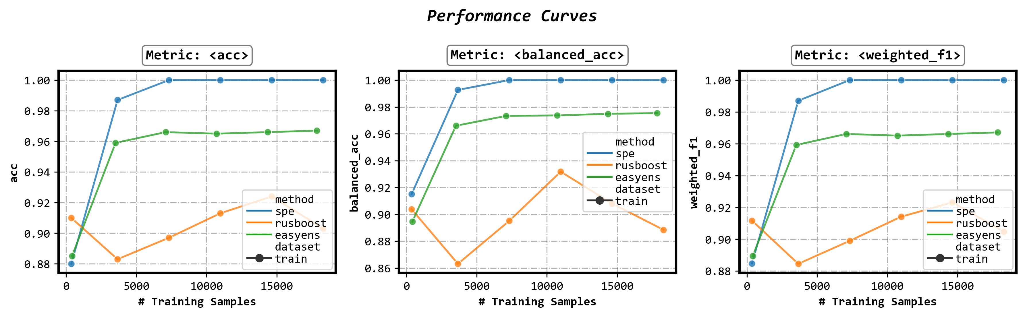
Plot performance curves
fig, axes = visualizer.performance_lineplot()
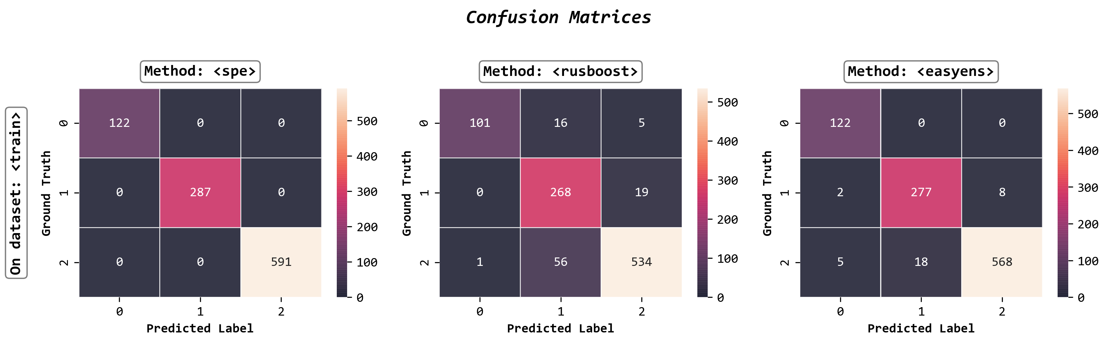
Plot confusion matrices
fig, axes = visualizer.confusion_matrix_heatmap()
Customizing training log
All ensemble classifiers in IMBENS support customizable training logging.
The training log is controlled by 3 parameters eval_datasets, eval_metrics, and training_verbose of the fit() method.
Read more details in the fit documentation.
Enable auto training log
clf.fit(..., train_verbose=True)
┏━━━━━━━━━━━━━┳━━━━━━━━━━━━━━━━━━━━━━━━━━┳━━━━━━━━━━━━━━━━━━━━━━━━━━━━━━━━━━━━┓
┃             ┃                          ┃            Data: train             ┃
┃ #Estimators ┃    Class Distribution    ┃               Metric               ┃
┃             ┃                          ┃  acc    balanced_acc   weighted_f1 ┃
┣━━━━━━━━━━━━━╋━━━━━━━━━━━━━━━━━━━━━━━━━━╋━━━━━━━━━━━━━━━━━━━━━━━━━━━━━━━━━━━━┫
┃      1      ┃ {0: 150, 1: 150, 2: 150} ┃ 0.838      0.877          0.839    ┃
┃      5      ┃ {0: 150, 1: 150, 2: 150} ┃ 0.924      0.949          0.924    ┃
┃     10      ┃ {0: 150, 1: 150, 2: 150} ┃ 0.954      0.970          0.954    ┃
┃     15      ┃ {0: 150, 1: 150, 2: 150} ┃ 0.979      0.986          0.979    ┃
┃     20      ┃ {0: 150, 1: 150, 2: 150} ┃ 0.990      0.993          0.990    ┃
┃     25      ┃ {0: 150, 1: 150, 2: 150} ┃ 0.994      0.996          0.994    ┃
┃     30      ┃ {0: 150, 1: 150, 2: 150} ┃ 0.988      0.992          0.988    ┃
┃     35      ┃ {0: 150, 1: 150, 2: 150} ┃ 0.999      0.999          0.999    ┃
┃     40      ┃ {0: 150, 1: 150, 2: 150} ┃ 0.995      0.997          0.995    ┃
┃     45      ┃ {0: 150, 1: 150, 2: 150} ┃ 0.995      0.997          0.995    ┃
┃     50      ┃ {0: 150, 1: 150, 2: 150} ┃ 0.993      0.995          0.993    ┃
┣━━━━━━━━━━━━━╋━━━━━━━━━━━━━━━━━━━━━━━━━━╋━━━━━━━━━━━━━━━━━━━━━━━━━━━━━━━━━━━━┫
┃    final    ┃ {0: 150, 1: 150, 2: 150} ┃ 0.993      0.995          0.993    ┃
┗━━━━━━━━━━━━━┻━━━━━━━━━━━━━━━━━━━━━━━━━━┻━━━━━━━━━━━━━━━━━━━━━━━━━━━━━━━━━━━━┛
Customize granularity and content of the training log
clf.fit(...,
        train_verbose={
            'granularity': 10,
            'print_distribution': False,
            'print_metrics': True,
        })
Click to view example output
┏━━━━━━━━━━━━━┳━━━━━━━━━━━━━━━━━━━━━━━━━━━━━━━━━━━━┓
┃             ┃            Data: train             ┃
┃ #Estimators ┃               Metric               ┃
┃             ┃  acc    balanced_acc   weighted_f1 ┃
┣━━━━━━━━━━━━━╋━━━━━━━━━━━━━━━━━━━━━━━━━━━━━━━━━━━━┫
┃      1      ┃ 0.964      0.970          0.964    ┃
┃     10      ┃ 1.000      1.000          1.000    ┃
┃     20      ┃ 1.000      1.000          1.000    ┃
┃     30      ┃ 1.000      1.000          1.000    ┃
┃     40      ┃ 1.000      1.000          1.000    ┃
┃     50      ┃ 1.000      1.000          1.000    ┃
┣━━━━━━━━━━━━━╋━━━━━━━━━━━━━━━━━━━━━━━━━━━━━━━━━━━━┫
┃    final    ┃ 1.000      1.000          1.000    ┃
┗━━━━━━━━━━━━━┻━━━━━━━━━━━━━━━━━━━━━━━━━━━━━━━━━━━━┛
Add evaluation dataset(s)
  clf.fit(...,
          eval_datasets={
              'valid': (X_valid, y_valid)
          })
Click to view example output
┏━━━━━━━━━━━━━┳━━━━━━━━━━━━━━━━━━━━━━━━━━━━━━━━━━━━┳━━━━━━━━━━━━━━━━━━━━━━━━━━━━━━━━━━━━┓
┃             ┃            Data: train             ┃            Data: valid             ┃
┃ #Estimators ┃               Metric               ┃               Metric               ┃
┃             ┃  acc    balanced_acc   weighted_f1 ┃  acc    balanced_acc   weighted_f1 ┃
┣━━━━━━━━━━━━━╋━━━━━━━━━━━━━━━━━━━━━━━━━━━━━━━━━━━━╋━━━━━━━━━━━━━━━━━━━━━━━━━━━━━━━━━━━━┫
┃      1      ┃ 0.939      0.961          0.940    ┃ 0.935      0.933          0.936    ┃
┃     10      ┃ 1.000      1.000          1.000    ┃ 0.971      0.974          0.971    ┃
┃     20      ┃ 1.000      1.000          1.000    ┃ 0.982      0.981          0.982    ┃
┃     30      ┃ 1.000      1.000          1.000    ┃ 0.983      0.983          0.983    ┃
┃     40      ┃ 1.000      1.000          1.000    ┃ 0.983      0.982          0.983    ┃
┃     50      ┃ 1.000      1.000          1.000    ┃ 0.983      0.982          0.983    ┃
┣━━━━━━━━━━━━━╋━━━━━━━━━━━━━━━━━━━━━━━━━━━━━━━━━━━━╋━━━━━━━━━━━━━━━━━━━━━━━━━━━━━━━━━━━━┫
┃    final    ┃ 1.000      1.000          1.000    ┃ 0.983      0.982          0.983    ┃
┗━━━━━━━━━━━━━┻━━━━━━━━━━━━━━━━━━━━━━━━━━━━━━━━━━━━┻━━━━━━━━━━━━━━━━━━━━━━━━━━━━━━━━━━━━┛
Customize evaluation metric(s)
from sklearn.metrics import accuracy_score, f1_score
clf.fit(...,
        eval_metrics={
            'acc': (accuracy_score, {}),
            'weighted_f1': (f1_score, {'average':'weighted'}),
        })
Click to view example output
┏━━━━━━━━━━━━━┳━━━━━━━━━━━━━━━━━━━━━━┳━━━━━━━━━━━━━━━━━━━━━━┓
┃             ┃     Data: train      ┃     Data: valid      ┃
┃ #Estimators ┃        Metric        ┃        Metric        ┃
┃             ┃  acc    weighted_f1  ┃  acc    weighted_f1  ┃
┣━━━━━━━━━━━━━╋━━━━━━━━━━━━━━━━━━━━━━╋━━━━━━━━━━━━━━━━━━━━━━┫
┃      1      ┃ 0.942      0.961     ┃ 0.919      0.936     ┃
┃     10      ┃ 1.000      1.000     ┃ 0.976      0.976     ┃
┃     20      ┃ 1.000      1.000     ┃ 0.977      0.977     ┃
┃     30      ┃ 1.000      1.000     ┃ 0.981      0.980     ┃
┃     40      ┃ 1.000      1.000     ┃ 0.980      0.979     ┃
┃     50      ┃ 1.000      1.000     ┃ 0.981      0.980     ┃
┣━━━━━━━━━━━━━╋━━━━━━━━━━━━━━━━━━━━━━╋━━━━━━━━━━━━━━━━━━━━━━┫
┃    final    ┃ 1.000      1.000     ┃ 0.981      0.980     ┃
┗━━━━━━━━━━━━━┻━━━━━━━━━━━━━━━━━━━━━━┻━━━━━━━━━━━━━━━━━━━━━━┛
About imbalanced learning
Class-imbalance (also known as the long-tail problem) is the fact that the classes are not represented equally in a classification problem, which is quite common in practice. For instance, fraud detection, prediction of rare adverse drug reactions and prediction gene families. Failure to account for the class imbalance often causes inaccurate and decreased predictive performance of many classification algorithms. Imbalanced learning aims to tackle the class imbalance problem to learn an unbiased model from imbalanced data.
For more resources on imbalanced learning, please refer to awesome-imbalanced-learning.
Acknowledgements
IMBENS was initially developed on top of imbalanced-learn, but has undergone heavy developments to implement many important imbalanced ensemble techniques. The infrastructure also underwent significant refactoring to support advanced ensemble learning features that are essential to practical usability (fine-grained training control, parallel computing, multi-class support, training logs, visualization, etc).
References
| # | Reference |
|---|---|
| [1] | Zhining Liu, Wei Cao, Zhifeng Gao, Jiang Bian, Hechang Chen, Yi Chang, and Tie-Yan Liu. 2019. Self-paced Ensemble for Highly Imbalanced Massive Data Classification. 2020 IEEE 36th International Conference on Data Engineering (ICDE). IEEE, 2020, pp. 841-852. |
| [2] | X.-Y. Liu, J. Wu, and Z.-H. Zhou, Exploratory undersampling for class-imbalance learning. IEEE Transactions on Systems, Man, and Cybernetics, Part B (Cybernetics), vol. 39, no. 2, pp. 539–550, 2009. |
| [3] | Chen, Chao, Andy Liaw, and Leo Breiman. “Using random forest to learn imbalanced data.” University of California, Berkeley 110 (2004): 1-12. |
| [4] | C. Seiffert, T. M. Khoshgoftaar, J. Van Hulse, and A. Napolitano, Rusboost: A hybrid approach to alleviating class imbalance. IEEE Transactions on Systems, Man, and Cybernetics-Part A: Systems and Humans, vol. 40, no. 1, pp. 185–197, 2010. |
| [5] | Maclin, R., & Opitz, D. (1997). An empirical evaluation of bagging and boosting. AAAI/IAAI, 1997, 546-551. |
| [6] | N. V. Chawla, A. Lazarevic, L. O. Hall, and K. W. Bowyer, Smoteboost: Improving prediction of the minority class in boosting. in European conference on principles of data mining and knowledge discovery. Springer, 2003, pp. 107–119 |
| [7] | S. Wang and X. Yao, Diversity analysis on imbalanced data sets by using ensemble models. in 2009 IEEE Symposium on Computational Intelligence and Data Mining. IEEE, 2009, pp. 324–331. |
| [8] | Fan, W., Stolfo, S. J., Zhang, J., & Chan, P. K. (1999, June). AdaCost: misclassification cost-sensitive boosting. In Icml (Vol. 99, pp. 97-105). |
| [9] | Shawe-Taylor, G. K. J., & Karakoulas, G. (1999). Optimizing classifiers for imbalanced training sets. Advances in neural information processing systems, 11(11), 253. |
| [10] | Viola, P., & Jones, M. (2001). Fast and robust classification using asymmetric adaboost and a detector cascade. Advances in Neural Information Processing System, 14. |
| [11] | Freund, Y., & Schapire, R. E. (1997). A decision-theoretic generalization of on-line learning and an application to boosting. Journal of computer and system sciences, 55(1), 119-139. |
| [12] | Breiman, L. (1996). Bagging predictors. Machine learning, 24(2), 123-140. |
| [13] | Guillaume Lemaître, Fernando Nogueira, and Christos K. Aridas. Imbalanced-learn: A python toolbox to tackle the curse of imbalanced datasets in machine learning. Journal of Machine Learning Research, 18(17):1–5, 2017. |
Related Projects
Check out Zhining's other open-source projects!
 Imbalanced Learning [Awesome] 
|
 Machine Learning [Awesome] 
|
 Self-paced Ensemble [ICDE] 
|
 Meta-Sampler [NeurIPS] 
|
Contributors ✨
Thanks goes to these wonderful people (emoji key):
 Zhining Liu 💻 🤔 🚧 🐛 📖 |
 leaphan 🐛 |
 hannanhtang 🐛 |
 H.J.Ren 🐛 |
 Marc Skov Madsen 🐛 |
This project follows the all-contributors specification. Contributions of any kind welcome!
