======== Grandalf

Graph and drawing algorithms framework

.. image:: https://travis-ci.org/bdcht/grandalf.svg?branch=master :target: https://travis-ci.org/bdcht/grandalf

.. image:: https://img.shields.io/lgtm/grade/python/g/bdcht/grandalf.svg?logo=lgtm&logoWidth=18 :target: https://lgtm.com/projects/g/bdcht/grandalf/context:python :alt: Code Quality

.. image:: https://img.shields.io/pypi/dm/grandalf.svg :target: https://pypi.python.org/pypi/grandalf

+-----------+--------------------------------------+ | Status: | Under Development | +-----------+--------------------------------------+ | Location: | https://github.com/bdcht/grandalf | +-----------+--------------------------------------+ | Version: | 0.8 | +-----------+--------------------------------------+

Description

Grandalf is a python package made for experimentations with graphs drawing algorithms. It is written in pure python, and currently implements two layouts: the Sugiyama hierarchical layout and the force-driven or energy minimization approach. While not as fast or featured as graphviz_ or other libraries like OGDF_ (C++), it provides a way to walk and draw graphs no larger than thousands of nodes, while keeping the source code simple enough to make it possible to easily tweak and hack any part of it for experimental purpose. With a total of about 1500 lines of python, the code involved in drawing the Sugiyama (dot) layout fits in less than 600 lines. The energy minimization approach is comprised of only 250 lines!

Grandalf does only 2 not-so-simple things:

• computing the nodes (x,y) coordinates (based on provided nodes dimensions, and a chosen layout)
• routing the edges with lines or nurbs

It doesn't depend on any GTK/Qt/whatever graphics toolkit. This means that it will help you find where to draw things like nodes and edges, but it's up to you to actually draw things with your favorite graphics toolkit.

Screenshots and Videos

See examples listed in the Wiki_.

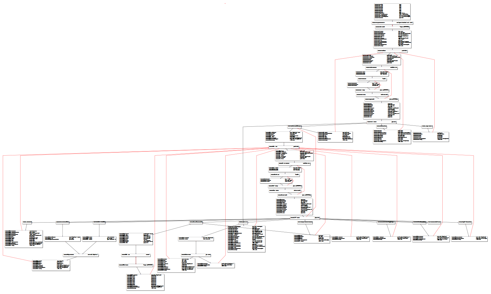
Here is a screenshot showing the result of rendering the control flow graph of a function:

.. image:: https://raw.github.com/bdcht/grandalf/master/doc/screenshot-1.png

Install

Grandalf suggests the following python packages:

• http://pypi.python.org/pypi/numpy, for the directed-constrained layout
• http://www.dabeaz.com/ply, for importing graphs from graphviz_ dot files.

Quickstart

Look for examples in tests/. Here is a very simple example:

.. code-block:: python

from grandalf.graphs import Vertex,Edge,Graph,graph_core V = [Vertex(data) for data in range(10)] X = [(0,1),(0,2),(1,3),(2,3),(4,0),(1,4),(4,5),(5,6),(3,6),(3,7),(6,8), ... (7,8),(8,9),(5,9)] E = [Edge(V[v],V[w]) for (v,w) in X] g = Graph(V,E) g.C [<grandalf.graphs.graph_core at 0x7fb23a95e4c0>] print([v.data for v in g.path(V[1],V[9])]) [1, 4, 5, 9] g.add_edge(Edge(V[9],Vertex(10))) <grandalf.graphs.Edge object at 0x7fb23a95e3a0> g.remove_edge(V[5].e_to(V[9])) <grandalf.graphs.Edge object at 0x7fb23a95e0a0> print([v.data for v in g.path(V[1],V[9])]) [1, 3, 6, 8, 9] g.remove_vertex(V[8]) <grandalf.graphs.Vertex object at 0x7fb23a933dc0> len(g.C) 2 print(g.path(V[1],V[9])) None for e in g.C[1].E(): print("%s -> %s"%(e.v[0].data,e.v[1].data)) ... 9 -> 10 from grandalf.layouts import SugiyamaLayout class defaultview(object): ... w,h = 10,10 ... for v in V: v.view = defaultview() ... sug = SugiyamaLayout(g.C[0]) sug.init_all(roots=[V[0]],inverted_edges=[V[4].e_to(V[0])]) sug.draw() for v in g.C[0].sV: print("%s: (%d,%d)"%(v.data,v.view.xy[0],v.view.xy[1])) ... 4: (30,65) 5: (30,95) 0: (0,5) 2: (-30,35) 1: (15,35) 3: (-15,65) 7: (-30,95) 6: (15,125) for l in sug.layers: ... for n in l: print(n.view.xy,end='') ... print('') ... (0.0, 5.0) (-30.0, 35.0)(15.0, 35.0)(45.0, 35.0) (-15.0, 65.0)(30.0, 65.0) (-30.0, 95.0)(0.0, 95.0)(30.0, 95.0) (15.0, 125.0) for e,d in sug.ctrls.items(): ... print('long edge %s --> %s points:'%(e.v[0].data,e.v[1].data)) ... for r,v in d.items(): print("%s %s %s"%(v.view.xy,'at rank',r)) ... long edge 3 --> 6 points: (-15.0, 65.0) at rank 2 (15.0, 125.0) at rank 4 (0.0, 95.0) at rank 3 long edge 4 --> 0 points: (0.0, 5.0) at rank 0 (30.0, 65.0) at rank 2 (45.0, 35.0) at rank 1

Overview

graph.py

Contains the "mathematical" methods related to graphs. This module defines the classes:

• Vertex (and vertex_core)
• Edge (and edge_core)
• Graph (and graph_core)

Vertex.

A Vertex object is defined by a data field holding whatever you want
associated to that vertex. It inherits from a vertex_core that --- when the
Vertex is added into a graph --- is holding the list of edges connected to
this Vertex and provides all methods associated to the properties of the
vertex inside the graph (degree, list of neigbors, list of input edges,
output edges, etc).
Of course, unless a Vertex belongs to a graph, all properties are empty or
None.
Example:

.. code-block:: python

 >>> v1 = Vertex('a')
 >>> v2 = Vertex('b')
 >>> v3 = Vertex('c')
 >>> v1.data
 'a'

Edge.
~~~~~
An Edge is defined by a pair of Vertex objects. If the graph is directed, the
direction of the edge is induced by the e.v list order otherwise the order is
irrelevant. See Usage section for details.
Example:

.. code-block:: python

 >>> e1 = Edge(v1,v2)
 >>> e2 = Edge(v1,v3,w=2)

Optional arguments includes a weight (defaults to 1) and a data holding
whatever you want associated with the edge (defaults to None). Edge weight
are used by the Dijkstra algorithm for finding 'shortest' paths with
respect to these weights.

graph_core.

A graph_core is used to hold a connected graph only. If the graph is not connected (ie there exists two vertex that can't be connected by an undirected path), then an exception is raised. Use of the Graph class is preferable unless you really know that your graph is connected. Example:

.. code-block:: python

g = graph_core([v1,v2,v3],[e1,e2])

The graph object can be updated by g.add_edge(e), g.remove_edge(e) or g.remove_vertex(v) which all raise an exception if connectivity is lost. Note that add_edge() will possibly extend the graph's vertex set with at most one new Vertex found in the added edge. See the Usage section for further details.

Graph.

This is the main class for graphs. The resulting graph is stored as "Disjoint
Sets" by processing the input lists of Vertex and Edge objects into a list of
graph_core components.
Example:

.. code-block:: python

 >>> v4,v5 = Vertex(4),Vertex(5)
 >>> g = Graph([v1,v2,v3,v4],[e1,e2])

The graph object can be updated by g.add_vertex(v), g.add_edge(e),
g.remove_vertex(v) and g.remove_edge(e) which all may result in updating a
graph_core, creating a new graph_core, or removing a graph_core from the
graph's internal list.

*layouts.py*
------------
Contains the "drawing" algorithms.
This module defines the classes:

- Layer
- SugiyamaLayout
- DigcoLayout

SugiyamaLayout.

This class performs a 2D hierarchical placement of a connected graph. The algorithm works only for directed acyclic graphs (DAG), so that a "feedback acyclic set" of edges is needed. To create a graph layout, you need to provide:

• a graph_core object where every Vertex has been equiped with a '.view' interface providing the width and height of the graphical representation of the Vertex (in our terminology, a Vertex equiped with a '.view' is a "node" of the graph)

To initiate the drawing (init_all) you will optionally provide:

• the list of "root" nodes
• the list of feedback acyclic edges
• constraint parameter related to how inverted edges are routed

In order to minimize edge crossings between each consecutive layers, the algorithm uses several rounds of nodes reordering (draw(N)). Increasing this parameter N can lead to layout with less crossings. For educational or debugging purpose, the drawing computation can be observed step-by-step (draw_step).

DigcoLayout.

This class performs a 2D hierarchical placement of a connected graph.
The main difference with SugiyamaLayout is that this algorithm is based on
optimization theory rather than on heuristics. It computes the node
coordinates by minimization of an "energy" function that describes the stress
factor associated to a layout.
This approach allows to take into account new constraints on node placement.
To create a graph layout, you only need to provide:
- a graph_core object where every Vertex has been equiped with a '.view'

*routing.py*
------------
Contains the edge routing algorithms.
This module defines the classes and functions:

- EdgeViewer
- route_with_lines
- route_with_splines

EdgeViewer.
~~~~~~~~~~~
This class provides a default 'view' for edges. Edges with no view will be
ignored by the draw_edge method of the layouts. If a view is provided it must
be equiped with a 'setpath' method to which a list of waypoints will be
passed.

route_with_lines.

This function allows to adjust the waypoints of the edge. It allows to draw a poly-line edge going through all points computed by the layout engine and adjusts the tail head position on the boundary of their nodes and precomputes the head angle. To use this routing method, set the route_edge field of the layout instance to this function (sug.route_edge = route_with_lines).

route_with_splines.

This function allows to draw edges by a combination of lines and bezier
curves. The curves are computed such that corners of a poly-line edge given
by route_with_lines are rounded.
To use this routing method,  set the route_edge field of the layout instance
to this function (sug.route_edge = route_with_splines) and use the values
returned in the .splines field of the edge view :
- an array of 2 points defines a line
- an array of 4 points defines a bezier curve.

*utils.py*
----------
Provides utilities like partially ordered sets, linear programming solvers,
parsers for external formats (Dot, etc.)
This module defines :

- Poset
- Dot

and some general purpose functions like:

- intersect2lines
- intersectR
- getangle (computing the atan2 value for directed edge heading)
- intersectC
- setcurve (computing a nurbs locally interpolating a given set of points)
- setroundcorner

Poset.
~~~~~~
This class is used by graph_core for both efficiently detecting if a Vertex
or Edge is in a graph (using builtin set()) and ensuring that elements of
the set are iterated always in the same order (using builtin list()).
Basically, a Poset is pair (set,list) that is kept synchronized.

Dot.
~~~~
This class contains a PLY lexer and parser for the graphviz dot format.
The parser reads all graphs currently defined in graphviz_
``graphs/{directed,undirected}/*.gvi``
as well as the dg.dot and ug.dot databases (> 5000 graphs parsed OK)
including *latin1* and *utf8* support (see russian.gv or Latin1.gv).

setcurve.
~~~~~~~~~
This function is used internally for edge routing. It is based on an method
described in "The NURBS Book" (Les A. Piegl, Wayne Tiller, Springer 1997)
implementing local interpolation of a given set of points with a set of
non-uniform b-splines of degree 3. The non-uniform knots are ignored.

setroundcorner.
~~~~~~~~~~~~~~~
This function uses setcurve to smooth the polyline edge at each corner. This
method provides the best result for edge routing with the SugiyamaLayout.
It is used in the route_with_splines function in routing.py.

*tests/*
--------
Contains many testing procedures as well as some graph samples.


Usage and Pitfalls
==================

Rather than an exhaustive library reference with all methods for all classes,
(see Python help() for that) we focus on a typical usage of grandalf and try to
also emphasize important notes.


Graph creation
--------------

Lets start by creating an empty graph:

.. code-block:: python

 >>> g = Graph()

Wether you first create the graph and add elements in it or create it after all
Vertex and Edge objects have been defined, is up to you.
For the moment the graph has no components :

.. code-block:: python

 >>> g.order()
 0
 >>> g.C
 []

Lets create some vertices now.

.. code-block:: python

 >>> v1 = Vertex('a')
 >>> v2 = Vertex('b')
 >>> v3 = Vertex()
 >>> v3.data = 'c'
 >>> v1.data
 'a'

First, note that the 'data' field is optional and can be added anytime in the
vertex. We are associating a string to this field so that it is easy to
identify a given vertex, but keep in mind that this data is not needed for
graph computations and drawings.
For the moment, the vertex objects are "free" in the sense that they are not
associated with any graph_core object. When a vertex belongs to a graph_core,
the reference to this graph_core is found in the 'c' field (component field).

To insert a Vertex in a Graph object we do:

.. code-block:: python

 >>> g.add_vertex(v1)

or we can add a new edge, then any new vertex it the edge will be attached to
the graph also:

.. code-block:: python

 >>> e1 = Edge(v1,v2)
 >>> e2 = Edge(v1,v3,w=2)
 >>> g.add_edge(e1)
 >>> g.add_edge(e2)
 >>> v2 in g.C[0]
 True

Warning: Vertex and Edge objects MUST belong to only one graph_core object at a
time. So you should never use the same Vertex/Edge into another graph without
removing it first from the current one !
Of course, removing a vertex also removes all edges linked to it.

.. code-block:: python

 >>> g.remove_vertex(v1)
 >>> e1 in g
 False
 >>> len(g.C)
 3

Removing v1 here has removed e1 and e2, and the graph g is now cut in 3
components holding each one vertex only. Lets rebuild the graph and extend it:

.. code-block:: python

 >>> g.add_edge(e1)
 >>> g.add_edge(e2)
 >>> v4,v5 = Vertex(4),Vertex(5)
 >>> g.add_edge(Edge(v4,v5))

Now g has two graph_core objects in g.C, and if

.. code-block:: python

 >>> g.add_edge(Edge(v5,v3))

the cores are merged in one component only.


Graph drawing
-------------

There are many possible layouts when it comes to graph drawings.
The current layout implemented is a hierarchical 2D layout suited for
*directed* graphs based on an method proposed by Sugiyama et al.
Our implementation is derived from the paper by Brandes & Kopf (GD 2001.)
This method is quite efficient but is based on many heuristics that are not
easy to tweak when you want to add some constraints like for example
"I want that nodes with property P to be placed near each others."

The "dig-cola" method is based on a different approach where graph properties
are expressed as constraints on node's coordinates, reducing the problem to
solving a set of inequalities with unknowns being the x,y coords of every
nodes. With this approach, adding new contraints is very simple.
The dig-cola method is implemented in old commits and is currently being
rewritten to match the design of SugiyamaLayout.

In Grandalf, a layout engine only applies on a graph_core object.
Basically drawing a Graph() requires that you draw all its connex components
and decide how to organize the entire drawing by moving each component where
you want. Since some methods involve "dummy" nodes inserted in the graph, it is
important to note that layout classes are completely separated from the
original : the underlying graph_core topology is never permanently modified.
This means that redrawing a graph for whatever reason (vertex added, edges
added, etc) is as simple as creating a new layout instance.
Of course, if you know what you are doing, you can try to update the drawing
based on the current layout instance but unless modifications of the topology
are very simple, this can be very difficult (enhancing this adaptative drawing
part is definetly in the TODO list!).

Before creating a layout engine associated with a graph_core, each vertex MUST
be equiped with what we call a 'view'. For a vertex v, such view must be an
object with attributes

- ``w`` (width) and
- ``h`` (height),
- ``xy`` (position)

and the layout engine will set the v.view.xy field with a (x,y) tuple value
corresponding to the center of the node.
In practice, this allows to use ``view`` objects that inherits from graphic
widgets (e.g. a rectangle in a Canvas) which will position the widget in the
canvas when the xy attribute is set.

If you want the layout to perform also edge routing, you MAY equipe edges also
with a 'view' attribute. For an edge e, the view must have a ``setpath`` method
taking a list of points as argument.
The layout engine will provide the list of (x,y) routing points, starting by
the ``e.v[0].view.xy``, then all intermediate dummy vertices position through
which the edge drawing should go, including the e.v[1].view.xy last point.
The routing.py module provides enhanced routing functions as well as a
representative EdgeViewer class to help finding the exact position where
drawing the 'tail' or the 'arrowhead' or define a set of splines made of Bezier
curves so that almost any curve Canvas primitive can be used.


SugiyamaLayout
~~~~~~~~~~~~~~
The Sugiyama layout draws a graph by separating the nodes in several layers.
These layers are stacked one under the others. The first layer contains the
"root" nodes.

the root nodes and the feedback edges sets
++++++++++++++++++++++++++++++++++++++++++
Most of the time, you don't need to bother with these notions because
init_all() will find the needed root nodes and feedback edges. Still, in some
cases it may help to know about these essential sets:

The Sugiyama layout is made for directed acyclic graphs. So the first requirement
for this layout is to have the list of inverted edges
(aka the feedback acyclic set needed to make the graph acyclic when needed.)
These edges are inverted in the graph_core only during some specific operations
and are reverted immediately after these computations.
For example, the graph is made acyclic for ranking the nodes into hierarchical
layers.
The graph_core class contains a method that computes the "strongly connected
sets" of the graph_core by using the Tarjan algorithm (get_scs_with_feedback).
A strongly connected set is a subset of vertex where for any two vertices A B,
there exist a directed path from A to B.
Of course a cycle is a strongly connected set, but such set may contain several
interlaced cycles. The algorithm constructs the "feedback acyclic set" by
tagging the edges with the 'feedback' field set to True. It performs a DFS
starting from the given set of nodes.
A good choice is of course to start with the set of nodes that have no incoming
edges, but if this set is empty (because the graph is cyclic) you will have to
choose a preferred set :
Hence,

.. code-block:: python

 >>> r = filter(lambda x: len(x.e_in())==0, gr.sV)
 >>> if len(r)==0: r = [my_guessed_root_node]
 >>> L = gr.get_scs_with_feedback(r)
 >>> inverted_edges=filter(lambda x:x.feedback, gr.sE)

leads to L containing the SCS of the ``gr`` component, and the feedback set is
then obtained by filter edges with the feedback flag.

As mentioned before, drawing with the SugiyamaLayout engine also requires that
you provide the list of "root" nodes.
Its up to you to decide which nodes are the "roots", but the natural definition
is as stated before :

.. code-block:: python

 >>> gr = g.C[0]
 >>> r = filter(lambda x: len(x.e_in())==0, gr.sV)

that is, the list r of vertex with no incoming edges.
Warning: if r is empty, you might want to use the set of edges computed before
to temporarily remove cycles and retry (look at ``__edge_inverter`` method.)

the init_all() and draw() methods
+++++++++++++++++++++++++++++++++
Drawing the gr component by computing .view.xy coordinates just resumes to:

.. code-block:: python

 >>> sug = SugiyamaLayout(gr)
 >>> sug.init_all()
 >>> sug.draw()

This will perform ONE round of the drawing algorithm. A single
round means that the node placement has been performed from the top layer to the
bottom layer and back to top. This may not be sufficient to reduce the edge
crossings, so you can draw again or simply provide the number of pass to
perform:

.. code-block:: python

 >>> sug.draw(3)

If you want to be able to draw the graph while the engine is running, you can
use the draw_step() iterator which yields at each layer during the forward and
backward trip.

Then, drawing the graph with a graphical canvas can be done by drawing each
views at their xy positions and either defining a ``setpath`` method that will
be called by grandalf draw_edges() with a set of routing points, or by using
predefined functions in ``routing.py`` like ``route_with_lines`` or
``route_with_splines``.

If you have installed masr_, just do:

.. code-block:: bash

 $ cd /path/to/grandalf
 $ ./masr-graph tests/samples/brandes.dot

When a node is focused, the SPACE key is bound to draw_step().next(). This
will show how the algorithm tries to reduce edge crossing in each layer by
modifying the layer ordering. Modified nodes will appear with green shadow.
The P key will cycle through the 4 internal alignment policies
(top-left, top-right, bottom-left, bottom-right.)

Optionally, inverted edges can be constrained to always start from the bottom
of their init vertex, and end on the top of their terminal vertex.

.. code-block:: bash

 $ ./masr-graph tests/samples/manhattan1.dot -ce


DigcoLayout
~~~~~~~~~~~
The DigcoLayout stands for "Directed Graph Constrained Layout". The method was
proposed by Dwyer & Koren in a paper presented at InfoVis 2005. It relies on
a stress minimization approach (similar to force-driven layouts like /neato/)
with hierarchical properties taken into account as additional constraints on
node coordinates.

the init_all() and draw() methods
+++++++++++++++++++++++++++++++++
Like for SugiyamaLayout, just do for example:

.. code-block:: python

 >>> dco = DigcoLayout(gr)
 >>> dco.init_all()
 >>> dco.draw(limit=100)

The init_all() method will take into account hierarchical information if the
graph is directed, and will randomly choose an initial distribution of node
coordinates. The draw() method will then converge towards the optimal solution
by using a conjugate-gradient method.
The ``limit`` parameter (defaults to gr.order() if not provided,) controls the
maximum iteration count of the convergence loop.
FIXME: In the current implementation, hierarchical levels are not taken into
account as additional constraints.

If you have installed masr_, just do:

.. code-block:: bash

 $ cd /path/to/grandalf
 $ masr-graph -digco -N 25 tests/samples/circle.dot

Or, you may visualize each step of the convergence by:

.. code-block:: bash

 $ masr-graph -digco -N 1 tests/samples/circle.dot

Now mouse-focus one of the nodes and press SPACE to see the next iteration.
Check out the masr/plugins/graph code to see how it works!

TODO
====
- add hierarchical constraints in DigcoLayout to support directed graphs
- add support for GraphML format import/export
- add support for pgf/tikz export
- provide facilities for efficient (interactive) edge re-routing

FAQ
===
1. Why is there no 'add_vertex()' method in the graph_core class ?

 Because graph_core are connected graphs, only add_single_vertex() makes sense.
 If you want to add a vertex directly into a graph_core, the vertex must be
 connected with an edge to another vertex already in the graph_core
 (use add_edge()).
 However, if the graph is empty, the first vertex can be attached to the graph
 by using add_single_vertex().

.. _graphviz: https://www.graphviz.org/
.. _OGDF: https://ogdf.uos.de/
.. _amoco: https://github.com/bdcht/amoco
.. _masr: https://github.com/bdcht/masr
.. _Wiki: https://github.com/bdcht/grandalf/wiki