gnn-powerflow

This project investigates Graph Neural Network application in power system analysis. It is intended to compare the performance of Graph Neural Network (GNN) vs traditional Multi Layer Perceptron (MLP) model at the same model complexity. The main question is, does leveraging data topology improve model accuracy? The code is developed with pytorch framework in Jupyter Notebook IDE. Initially, the model is programmed in python from scratch. Midway, I utilize pytorch-geometric library to simplify the process and add more built-in optimizations. You can get a grasp of the main ideas of my thesis in the following explanation.

Integrating Power Grid Topology in Graph Neural Networks for Power Flow.

Recent advances in Neural Network (NN) offer an interesting opportunity to integrate graph topology in a Neural Network system. This framework is called Graph Neural Network (GNN). In power systems, an electrical power grid can be represented as a graph with high dimensional features and interdependency among buses. This perspective may offer a better state of the art machine learning for power systems analysis. This study seeks the opportunity to integrate power grid topology in the GNN framework for power flow application. A comparison between several GNN architectures with equivalent model complexities are discussed. The comparison is also done for various dataset sizes.

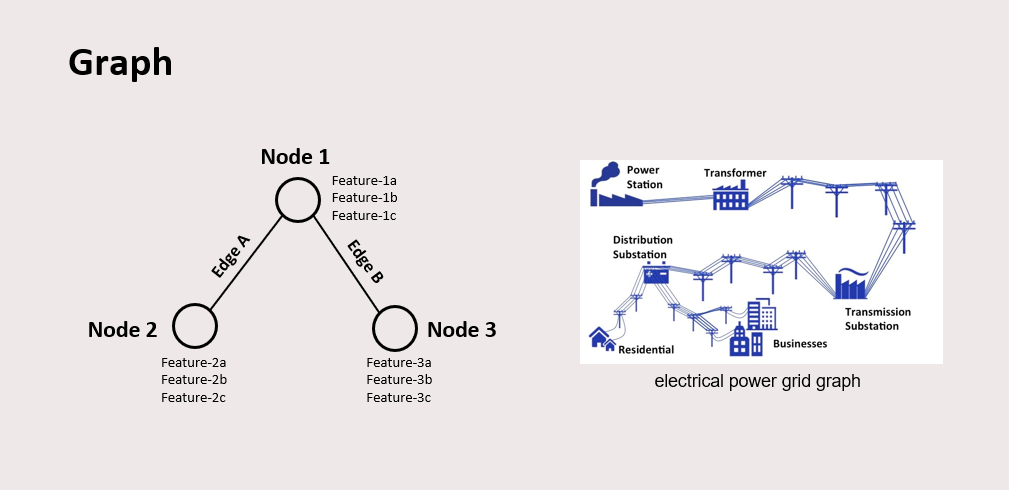
A graph is a structure consisting of nodes and edges. Nodes are the content of the data, and edges are the connectivity between these data. Graph is basically how the world represents itself, since many naturally generated data are in the shape of graphs: protein, social media, and also electrical power grid. In a power grid, the buses can be seen as the nodes, and the lines can be seen as the edges. The node features are voltage, voltage angle, active power, and reactive power, while the line features can be line current and line resistance.

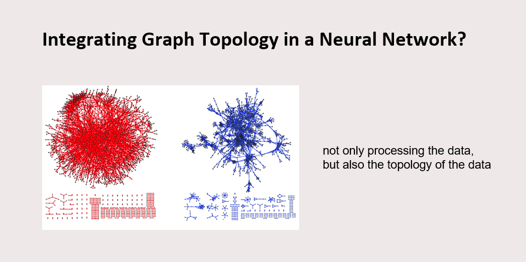
Traditional NN models like Multi Layer Perceptron (MLP) usually only process the content of the data. What if we can also utilize the structure information of the data? Would it improve the model accuracy? That is the main idea of GNN, where we also process the shape information of graph data. From the protein graph data, GNN can make use of the protein element as well as the protein structure.

In a power grid, a bus can be of type slack bus, pv bus, and pq bus. Every bus has known and unknown variables, e.g. PQ bus knows its active power P and reactive power Q, and does not know its voltage V and voltage angle d. Power flow tries to calculate the unknown variables using known variables as input using electrical formulas. GNN for power flow tries to predict the unknown variables by utilizing the known variables using a machine learning model.

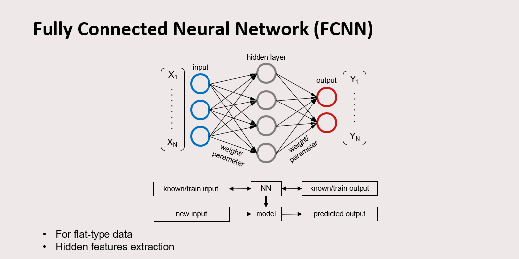
Fully Connected Neural Network (FCNN) is a supervised machine learning framework. It is built upon a set of known input and output, then makes a predictive model based on their relation. The lines that connect the nodes are weight or trainable parameters, because this value will be adjusted in the training. Every node value is multiplied with the parameter, until it becomes the predicted output. The difference of the predicted output and the ground truth is called the loss function, can be calculated using logistic regression for classification or mean squared error for regression. We tune the value of the parameter for some iteration until the prediction model is accurate enough. The process is called optimization. After the model is made, we can give it a new input and predict the output. FCNN is for flat type data. FCNN does hidden features extraction using its hidden layer.

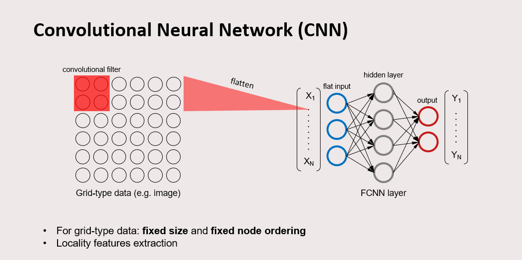
Convolutional Neural Network (CNN) is for grid-shaped data, a data type with fixed size and node ordering. For example, a digital image is a grid-shaped data that consists of pixels with fixed size of row and column, and has fixed node ordering. CNN firstly applies a convolutional filter to the data, then flatten its output, and later on pass it on to a FCNN layer. Flatten meaning that the data from any shape is made to be a 1 dimensional data. The convolution filter leverages the locality feature of the grid-type data.

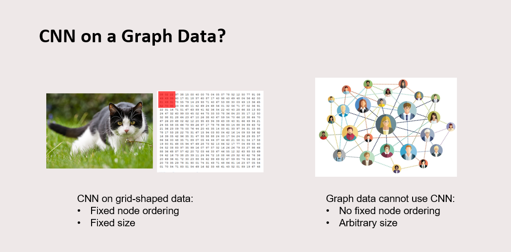
The question is, can CNN be applied to graph data? The answer is no, because CNN is only for data with fixed row and column and fixed node ordering like images, while graph data has no fixed node ordering. There has to be another way to embed a convolutional filter to graph data. That is where GNN comes in place.

The main principle of GNN is its message passing. It is a mechanism where a target node receives information from its neighboring nodes. E.g., node 4 as the target node will get messages from node 1, 5, and 6, and node 4 itself from the previous state. This message passing at node 4 happens at every node for 1 GNN layer. We apply a simple summation of the neighboring node’s message, then multiply it with trainable parameter W, then apply nonlinear activation function as the input for the next layer. But how to apply this mathematically?

We can do that using the adjacency matrix A. Adjacency matrix is a matrix that represents the mapping of neighboring nodes in graph data. For example, at the red box at the left, you can see the neighboring nodes of node 4. Its neighboring nodes are nodes 1, 4, 5, 6, so those columns will be assigned with value of 1, and the other column will be assigned with zero. If we multiply this row with the column of matrix data X, it will become a simple summation message passing.

A more advanced GNN type is Graph Convolution Network (GCN). The only difference with the previous GNN is that GCN implements averaging message passing. We can implement that by preprocessing the adjacency matrix A with the inverse of degree matrix D. A degree matrix is a matrix that denotes the number of neighbor for each node of a graph, e.g., because node 4 has 4 neighbors, then the 4th row will be divided by 4, and it becomes averaging message passing. We can set the row and column of W to determine how many features will be extracted in the next layer.

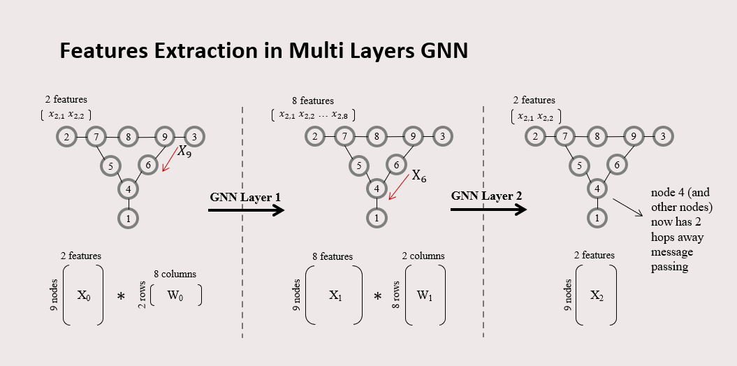
This is how hidden feature extraction is done in multi-layer GNN. Here, we applied 2 GNN layers to a graph data with 9 nodes. Initially, every node has 2 features. It is multiplied with parameter matrix W0 with 2 rows and 8 columns, and the output now has 8 features after applying the first GNN layer. After that, it is multiplied with matrix parameter W1 with 8 rows and 2 columns, and now every node has 2 features at the last state, after it is applied by the second GNN layer. Take a look at node 4 at the last state. This node 4 previously received information from node 6, and node 6 previously got information from node 9. This means, node 4 now has 2 hops away message passing, or 2 neighbors away information acquiring. So that means applying 2 layers of GNN is the same with 2 hops away GNN.

Just like CNN, GNN can also be seen as another layer of Deep Learning. We can apply the GNN layer to graph data, flatten the output, and make it an input to the FCNN layer.

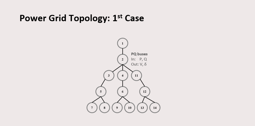
This is the first case of graph data I used, which consists of 14 nodes. Each node is a PQ bus.

This is the second case of the graph data. Now I add to the graph various sizes of loops: small loop, medium loop, and big loop. I want to check whether there is any effect of adding a loop to the performance of GNN.

These are the models to be compared in the experiment. I made 3 kinds of models. Model 1 consists of 2 traditional fully connected layers. Model 2 consists of 1 GNN layer continued by 1 fully connected layer. Model 3 consists of 2 GNN layers or 2 hops away GNN ended by a fully connected layer. The three models are designed to have a similar number of parameters, around 2600, because I want to compare the models at an equivalent level. The hyperparameters can be seen in the figure.

This is how I generate the dataset. I use DIgSILENT PowerFactory 2020. I made 102 datasets, and each dataset has 2000 data points. From these 102 datasets, I use 1 as train dataset, 1 as validation dataset, and 100 as test dataset.

This is the shape of 1 dataset. Each dataset has 2000 data points. Each data point consists of 14 rows from the 14 nodes of the graph data. Each node has 2 input features and 2 output features. If we want to use this data structure on fully connected networks, we must flatten it first.

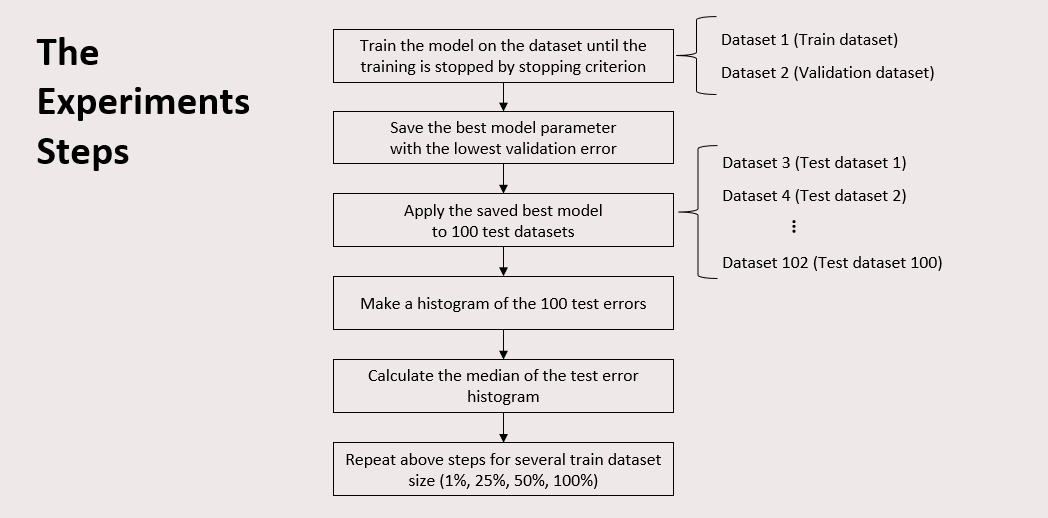
This is the experiment steps that I conducted. The complete result can be seen in the report document: https://github.com/mukhlishga/gnn-powerflow/blob/main/document/Integrating%20Power%20Grid%20Topology%20in%20Graph%20Neural%20Networks%20for%20Power%20Flow.pdf