evaluation-toolkit

You may use this toolkit to:

1. Evaluate light field algorithms
2. Validate a benchmark submission
3. Convert between depth and disparity maps
4. Convert between pfm and png files
5. Create figures
6. Create point clouds
7. Compute pixel offset

For details on how to prepare your submission for the 4D Light Field Benchmark, please read the submission instructions. Please don't hesitate to contact us for any kind of questions, feedback, or bug reports: contact at lightfield-analysis.net

Dependencies

The scripts are tested with Python 2.7. They require numpy, matplotlib, scikit-image, scipy and their respective dependencies as listed in the requirements.txt. We recommend using pip to install the dependencies:

$ pip install -r requirements.txt

Introduction

Per default, the toolkit expects the following file structure. You may adjust the settings.py if you prefer another setup.

|-- data
    |-- stratified
    |-- training
    |-- test
|-- algo_results
    |-- epi1
       |-- disp_maps
         |-- backgammon.pfm
         |-- boxes.pfm
         |-- ...
       |-- runtimes
         |-- backgammon.txt
         |-- ...
     |-- meta_data.json
|-- evaluation
|-- source

algo_results: Place the results and runtimes of our method into this directory to run the evaluation on your method. If you want to compare your results to other benchmark participants, download their disparity maps of the stratified and training scenes here (snapshot 10.07.2017) and place it next to your method.

data: Contains the config files for all scenes, but no light field data. If you want to run the evaluation please download the scene data from our website and place it into this directory. The easiest way is to download and extract the "benchmark.zip" from the list of download links that you receive via email.

evaluation: The target directory for scores and figures that will be created during the evaluation.

source: Contains the Python 2.7 source code. Feel free to adjust and extend it according to your needs.

How To

General Notes

For most scripts, you may pass your choice of scenes, algorithms and metrics as arguments. Per default, all available scenes and algorithms of the respective directories are used.

For all scripts, we refer to the usage for an extensive list of available options:

python any_toolkit_script.py -h

Please note that not all metrics are defined on all scenes, e.g. there is no Pyramids Bumpiness score on the Dino scene. Some evaluations require test scene ground truth (Bedroom, Bicycle, Herbs, Origami). Adjust your command line arguments accordingly, e.g. by using -s training stratified.

1. Evaluate light field algorithms

To evaluate all algorithms in the "algo_results" directory including all scenes, metrics, and visualizations, run:

python run_evaluation.py --visualize

This will compute the scores and figures that are also computed on the evaluation server of the benchmark website. To evaluate your method, copy your results next to the baseline algorithms in the "algo_results" directory. You may select any subset of algorithms, scenes, and metrics. For example:

python run_evaluation.py -a your_algo epi1 -s boxes cotton dino -m mse badpix007

2. Validate a benchmark submission

To validate your submission, run:

python validate_submission.py some/path/to/submission.zip

Please not that your zip archive should directly contain a disp_maps and a runtimes directory without any further nested directories. Check out the submission instructions for further details.

3. Convert between depth and disparity maps

Run convert_depth2disp.py and convert_disp2depth.py to convert between depth and disparity maps. You need to provide paths to the input and output map and to the scene parameter file.

The corresponding formulas are:

depth_mm = beta * focus_distance_mm / (disp_px * focus_distance_mm * sensor_size_mm + beta)

disp_px = (beta * focus_distance_mm / depth_mm - beta) / (focus_distance_mm * sensor_size_mm)
 
where beta = baseline_mm * focal_length_mm * max(width_px, height_px)

The config files provide the image width and height in pixels and the sensor size of the larger of both dimensions in mm.

4. Convert between pfm and png files

There a demo scripts convert_pfm2png.py and convert_png2pfm.py to show how to convert between pfm and png files of disparity maps. The scripts assume a png range of [0, 255] and use the [disp_min, disp_max] range of the scene as pfm range. You may need to adjust these ranges and the conversion, depending on your images.

5. Create figures

Metric overviews

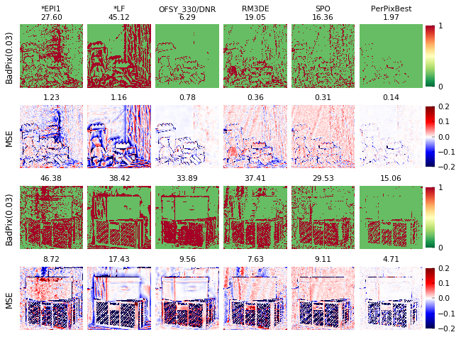
To create tables with metric visualizations and scores, run plot_metric_overview.py with the metrics, scenes, and algorithms of your choice. There will be one column per algorithm and one row per metric. If you select multiple scenes, they will be added as additional rows. You may also add meta algorithms such as the best disparity estimate per pixel.

Example:

python plot_metric_overview.py -m badpix003 mse -s dino boxes -a epi1 lf ofsy_330dnr rm3de spo -p best

Radar charts

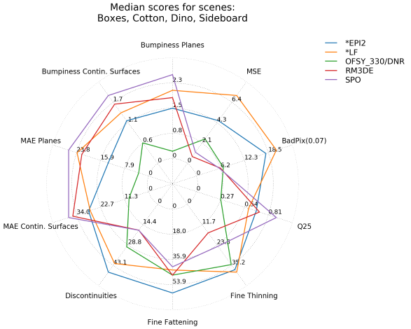
To create a radar chart, run plot_radar.py with the metrics, scenes, and algorithms of your choice. For each metric, the median of all applicable scenes is used per algorithm. Metrics which are not applicable for any of the given scenes (e.g. Pyramids Bumpiness on the training scenes) are omitted. For this chart, scores are read from the results.json of each algorithm. Run the run_evaluation.py to compute the required scores before creating the radar chart.

Example:

python plot_radar.py -m regions q25 badpix007 mse -s training -a epi2 lf ofsy_330dnr rm3de spo

Error heatmaps

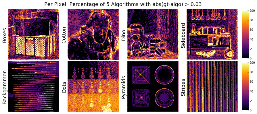
Error heatmaps highlight those regions where most of the given algorithms have difficulties. Per pixel, they depict the percentage of algorithms with an absolute disparity error above the given threshold.

Example:

python plot_error_heatmaps.py -t 0.03 -s stratified training

Meta algorithm comparisons

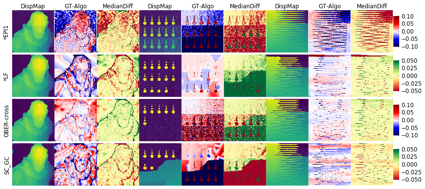
Run plot_meta_algo_comparisons.py with the algorithms, scenes and meta-algorithm of your choice. There will be one row per algorithm. Per scene, there will be three columns: the algorithm disparity map and the differences to the ground truth and to the meta algorithm.

Example:

python plot_meta_algo_comparisons.py -s cotton dots backgammon -a epi1 lf obercross sc_gc -p median_diff

Pairwise algorithm comparisons

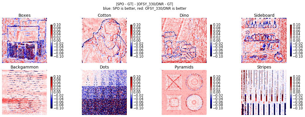
Use this visualization to highlight the strengths and weaknesses of one algorithm compared to a second algorithm.

Example:

python plot_pairwise_comparisons.py -a spo ofsy_330dnr -s training stratified

BadPix series

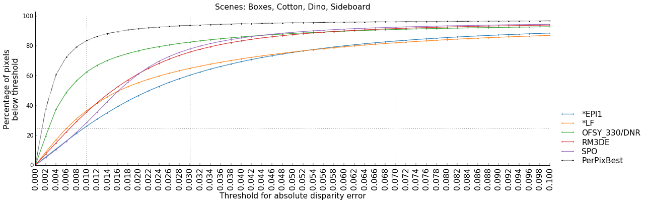
For this figure, BadPix percentages are displayed for a range of thresholds. The average percentage is used when multiple scenes are given.

Example:

python plot_bad_pix_series.py -s training -p best

Paper figures

To create equivalent figures to the figures in the ACCV 2016 or CVPRW 2017 paper, run:

python create_paper_figures_accv_2016.py
python create_paper_figures_cvprw_2017.py

Note that the best parameter setting per scene was chosen for the figures in the ACCV paper. For the benchmark, one setting for all scenes is required. Some of the provided baseline disparity maps may therefore differ from the results in the paper.

6. Create point clouds

Run export_pointloud.py to create ply files which you can open with MeshLab or other viewers. Apart from algorithms, you may also use -a gt to create a point cloud with the ground truth depth.

Example:

python export_pointloud.py -s dino -a epi1

If you want to convert any disparity map to a point cloud, run convert_disp2pointcloud.py. You need to provide paths to the disparity map and the camera parameter file. You may optionally provide a path to the corresponding image to add colors to your point cloud.

Example:

python convert_disp2pointcloud.py /path/to/dispmap.pfm /path/to/parameters.cfg /path/to/pointcloud.ply

7. Compute pixel offset

Our light fields are created with shifted cameras (see our supplemental material of the ACCV 2016 paper for details). The cameras have parallel optical axes but their sensors are shifted so that they see the same area of the scene. You can also think of it that the non-center views are moved by a certain amount of pixels. To compute this pixel offset for "one step" (between two adjacent views), run compute_offset.py with a list of scenes.

Example:

python compute_offset.py -s dino cotton

The corresponding formula is:

offset = baseline_mm * focal_length_mm / focus_dist_m / 1000. / sensor_mm * max(width, height)

License

This work is licensed under the Creative Commons Attribution-NonCommercial-ShareAlike 4.0 International License. To view a copy of this license, visit http://creativecommons.org/licenses/by-nc-sa/4.0/.

Authors: Katrin Honauer & Ole Johannsen

Website: www.lightfield-analysis.net

The 4D Light Field Benchmark was jointly created by the University of Konstanz and the HCI at Heidelberg University. If you use any part of the benchmark, please cite our paper "A dataset and evaluation methodology for depth estimation on 4D light fields". Thanks!

@inproceedings{honauer2016benchmark, title={A dataset and evaluation methodology for depth estimation on 4D light fields}, author={Honauer, Katrin and Johannsen, Ole and Kondermann, Daniel and Goldluecke, Bastian}, booktitle={Asian Conference on Computer Vision}, year={2016}, organization={Springer} }