Before going into a clean phase, we are retrieving the subject of the document from the text.
for i,txt in enumerate(news['content']):
    subject = re.findall('Subject:(.*\n)',txt)
    if (len(subject) !=0):
        news.loc[i,'Subject'] =str(i)+' '+subject[0]
    else:
        news.loc[i,'Subject'] ='NA'
df_news =news[['Subject','content']]
Now, we are removing the unwanted data from text content and the subject of a dataset.
df_news.content =df_news.content.replace(to_replace='from:(.*\n)',value='',regex=True) ##remove from to email
df_news.content =df_news.content.replace(to_replace='lines:(.*\n)',value='',regex=True)
df_news.content =df_news.content.replace(to_replace='[!"#$%&\'()*+,/:;?@[\\]^_`{|}~]',value=' ',regex=True) #remove punctuation except
df_news.content =df_news.content.replace(to_replace='-',value=' ',regex=True)
df_news.content =df_news.content.replace(to_replace='\s+',value=' ',regex=True)    #remove new line
df_news.content =df_news.content.replace(to_replace='  ',value='',regex=True)                #remove double white space
df_news.content =df_news.content.apply(lambda x:x.strip())  # Ltrim and Rtrim of whitespace
2.2 data preprocessing
Preprocessing is one of the major steps when we are dealing with any kind of text models. During this stage, we have to look at the distribution of our data, what techniques are needed and how deep we should clean.
Lowercase
Conversion the text into a lower form. i.e. ‘Dogs’ into ‘dogs’
df_news['content']=[entry.lower() for entry in df_news['content']]
Word Tokenization
Word tokenization is the process to divide the sentence into the form of a word.
“Jhon is running in the track” → ‘john’, ‘is’, ‘running’, ‘in’, ‘the’, ‘track’
df_news['Word tokenize']= [word_tokenize(entry) for entry in df_news.content]
Stop words
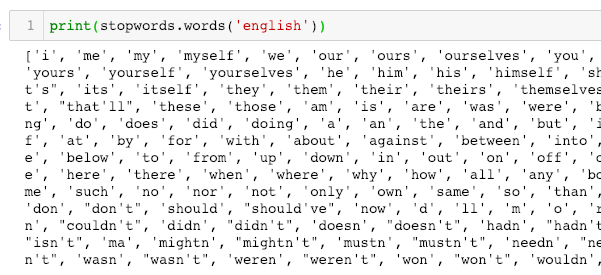
Stop words are the most commonly occurring words which don’t give any additional value to the document vector. in-fact removing these will increase computation and space efficiency. NLTK library has a method to download the stopwords.
Word Lemmatization
Lemmatisation is a way to reduce the word to root synonym of a word. Unlike Stemming, Lemmatisation makes sure that the reduced word is again a dictionary word (word present in the same language). WordNetLemmatizer can be used to lemmatize any word.
i.e. rocks →rock, better →good, corpora →corpus
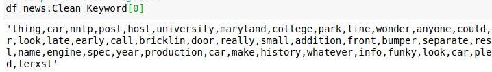
Here created wordLemmatizer function to remove a single character, stopwords and lemmatize the words.
# WordNetLemmatizer requires Pos tags to understand if the word is noun or verb or adjective etc. By default it is set to Noun
def wordLemmatizer(data):
    tag_map = defaultdict(lambda : wn.NOUN)
    tag_map['J'] = wn.ADJ
    tag_map['V'] = wn.VERB
    tag_map['R'] = wn.ADV
    file_clean_k =pd.DataFrame()
    for index,entry in enumerate(data):

        # Declaring Empty List to store the words that follow the rules for this step
        Final_words = []
        # Initializing WordNetLemmatizer()
        word_Lemmatized = WordNetLemmatizer()
        # pos_tag function below will provide the 'tag' i.e if the word is Noun(N) or Verb(V) or something else.
        for word, tag in pos_tag(entry):
            # Below condition is to check for Stop words and consider only alphabets
            if len(word)>1 and word not in stopwords.words('english') and word.isalpha():
                word_Final = word_Lemmatized.lemmatize(word,tag_map[tag[0]])
                Final_words.append(word_Final)
            # The final processed set of words for each iteration will be stored in 'text_final'
                file_clean_k.loc[index,'Keyword_final'] = str(Final_words)
                file_clean_k.loc[index,'Keyword_final'] = str(Final_words)
                file_clean_k=file_clean_k.replace(to_replace ="\[.", value = '', regex = True)
                file_clean_k=file_clean_k.replace(to_replace ="'", value = '', regex = True)
                file_clean_k=file_clean_k.replace(to_replace =" ", value = '', regex = True)
                file_clean_k=file_clean_k.replace(to_replace ='\]', value = '', regex = True)
    return file_clean_k
By using this function took around 13 hrs time to check and lemmatize the words of 11K documents of the 20newsgroup dataset. Find below the JSON file of the lemmatized word.
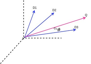
It is the most common metric used to calculate the similarity between document text from input keywords/sentences. Mathematically, it measures the cosine of the angle b/w two vectors projected in a multi-dimensional space.
Cosine Similarity b/w document to query
In the above diagram, have 3 document vector value and one query vector in space. when we are calculating the cosine similarity b/w above 3 documents. The most similarity value will be D3 document from three documents.
1. Document search engine with TF-IDF:
TF-IDF stands for “Term Frequency — Inverse Document Frequency”. This is a technique to calculate the weight of each word signifies the importance of the word in the document and corpus. This algorithm is mostly using for the retrieval of information and text mining field.
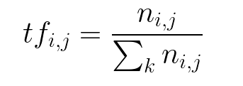
Term Frequency (TF)
The number of times a word appears in a document divided by the total number of words in the document. Every document has its term frequency.
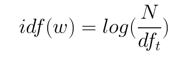
Inverse Data Frequency (IDF)
The log of the number of documents divided by the number of documents that contain the word w. Inverse data frequency determines the weight of rare words across all documents in the corpus.
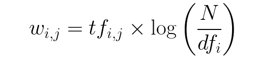
Lastly, the TF-IDF is simply the TF multiplied by IDF.
TF-IDF = Term Frequency (TF) * Inverse Document Frequency (IDF)
Rather than manually implementing TF-IDF ourselves, we could use the class provided by Sklearn.
Generated TF-IDF by using TfidfVectorizer from Sklearn
Import the packages:
import pandas as pd
import numpy as np
import os
import re
import operator
import nltk
from nltk.tokenize import word_tokenize
from nltk import pos_tag
from nltk.corpus import stopwords
from nltk.stem import WordNetLemmatizer
from collections import defaultdict
from nltk.corpus import wordnet as wn
from sklearn.feature_extraction.text import TfidfVectorizer
TF-IDF
from sklearn.feature_extraction.text import TfidfVectorizer
import operator## Create Vocabulary
vocabulary = set()for doc in df_news.Clean_Keyword:
    vocabulary.update(doc.split(','))vocabulary = list(vocabulary)# Intializating the tfIdf model
tfidf = TfidfVectorizer(vocabulary=vocabulary)# Fit the TfIdf model
tfidf.fit(df_news.Clean_Keyword)# Transform the TfIdf model
tfidf_tran=tfidf.transform(df_news.Clean_Keyword)
The above code has created TF-IDF weight of the whole dataset, Now have to create a function to generate a vector for the input query.
Create a vector for Query/search keywords
def gen_vector_T(tokens):Q = np.zeros((len(vocabulary)))
    x= tfidf.transform(tokens)
    #print(tokens[0].split(','))
    for token in tokens[0].split(','):
        #print(token)
        try:
            ind = vocabulary.index(token)
            Q[ind]  = x[0, tfidf.vocabulary_[token]]
        except:
            pass
    return Q
query_vector = gen_vector_T(q_df['q_clean']) for d in tfidf_tran.A: d_cosines.append(cosine_sim(query_vector, d))
out = np.array(d_cosines).argsort()[-k:][::-1] #print("") d_cosines.sort() a = pd.DataFrame() for i,index in enumerate(out): a.loc[i,'index'] = str(index) a.loc[i,'Subject'] = df_news['Subject'][index] for j,simScore in enumerate(d_cosines[-k:][::-1]): a.loc[j,'Score'] = simScore return a
Testing the function
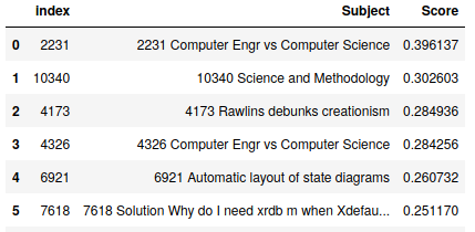
cosine_similarity_T(10,’computer science’)
Result of top 5 similarity documents for “computer science” word
2. Document search engine with Google Universal sentence encoder
Introduction Google USE
The pre-trained Universal Sentence Encoder is publicly available in Tensorflow-hub. It comes with two variations i.e. one trained with Transformer encoder and others trained with Deep Averaging Network (DAN). They are pre-trained on a large corpus and can be used in a variety of tasks (sentimental analysis, classification and so on). The two have a trade-off of accuracy and computational resource requirement. While the one with Transformer encoder has higher accuracy, it is computationally more expensive. The one with DNA encoding is computationally less expensive and with little lower accuracy.
Here we are using Second one DAN Universal sentence encoder as available in this URL:- Google USE DAN Model
Both models take a word, sentence or a paragraph as input and output a 512-dimensional vector.
A prototypical semantic retrieval pipeline, used for textual similarity.
import pandas as pd
import numpy as np
import re, string
import os
import tensorflow as tf
import tensorflow_hub as hub
import matplotlib.pyplot as plt
import seaborn as sns
from sklearn.metrics.pairwise import linear_kernel
Download the model from TensorFlow-hub of calling direct URL:
#Model load through local path:module_path ="/home/zettadevs/GoogleUSEModel/USE_4"
%time model = hub.load(module_path)#Create function for using model training
def embed(input):
    return model(input)
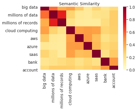
Use Case 1:- Word semantic
WordMessage =[‘big data’, ‘millions of data’, ‘millions of records’,’cloud computing’,’aws’,’azure’,’saas’,’bank’,’account’]
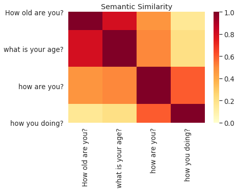
Use Case 2: Sentence Semantic
SentMessage =['How old are you?','what is your age?','how are you?','how you doing?']
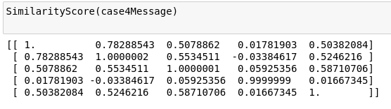
Use Case 3: Word, Sentence and paragram Semantic
word ='Cloud computing'Sentence = 'what is cloud computing'Para =("Cloud computing is the latest generation technology with a high IT infrastructure that provides us a means by which we can use and utilize the applications as utilities via the internet."
        "Cloud computing makes IT infrastructure along with their services available 'on-need' basis."
        "The cloud technology includes - a development platform, hard disk, computing power, software application, and database.")Para5 =(
    "Universal Sentence Encoder embeddings also support short paragraphs. "
    "There is no hard limit on how long the paragraph is. Roughly, the longer "
    "the more 'diluted' the embedding will be.")Para6 =("Azure is a cloud computing platform which was launched by Microsoft in February 2010."
       "It is an open and flexible cloud platform which helps in development, data storage, service hosting, and service management."
       "The Azure tool hosts web applications over the internet with the help of Microsoft data centers.")
case4Message=[word,Sentence,Para,Para5,Para6]
Training the model
Here we have trained the dataset at batch-wise because it takes a long time to execution to generate the graph of the dataset. so better to train batch-wise data.
def SearchDocument(query):
    q =[query]
    # embed the query for calcluating the similarity
    Q_Train =embed(q)

    #imported_m = tf.saved_model.load('/home/zettadevs/GoogleUSEModel/TrainModel')
    #loadedmodel =imported_m.v.numpy()
    # Calculate the Similarity
    linear_similarities = linear_kernel(Q_Train, con_a).flatten()
    #Sort top 10 index with similarity score
    Top_index_doc = linear_similarities.argsort()[:-11:-1]
    # sort by similarity score
    linear_similarities.sort()
    a = pd.DataFrame()
    for i,index in enumerate(Top_index_doc):
        a.loc[i,'index'] = str(index)
        a.loc[i,'File_Name'] = df_news['Subject'][index] ## Read File name with index from File_data DF
    for j,simScore in enumerate(linear_similarities[:-11:-1]):
        a.loc[j,'Score'] = simScore
    return a
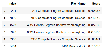
Test the search:
SearchDocument('computer science')
Conclusion:
At the end of this tutorial, we are concluding that “google universal sentence encoder” model is providing the semantic search result while TF-IDF model doesn’t know the meaning of the word. just giving the result based on words available on the documents.