Chrisding Seal Save

Code for Simultaneous Edge Alignment and Learning (SEAL)

Project README

Simultaneous Edge Alignment and Learning (SEAL)

By Zhiding Yu, Weiyang Liu, Yang Zou, Chen Feng, Srikumar Ramalingam, B. V. K. Vijayakumar and Jan Kautz

License

SEAL is released under the MIT License (refer to the LICENSE file for details).

Introduction
Citation
Requirements
Installation
Usage
Video Demo
Note
References
Contact

Introduction

The repository contains the entire pipeline (including data preprocessing, training, testing, label refine, evaluation, visualization, and demo generation, etc) for SEAL.

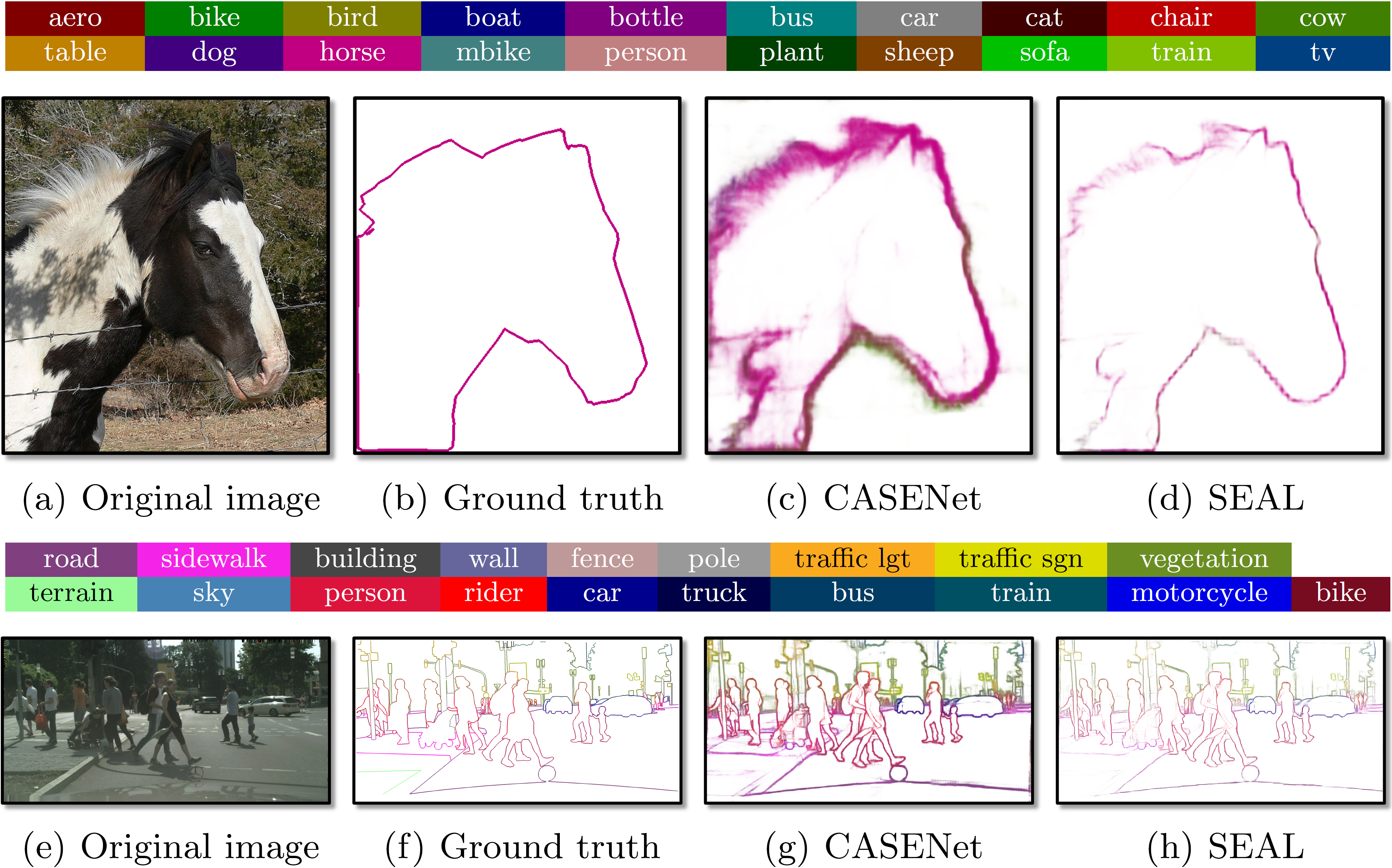
SEAL is a recently proposed learning framework towards edge learning under noisy labels. The framework seeks to directly generate high quality thin/crisp object semantic boundaries without any post-processing, by jointly performing edge alignment with edge learning. In particular, edge alignment is formulated as latent variable optimization and learned end-to-end during network training. For more details, please refer to the arXiv technical report and the ECCV18 paper. We highly recommend the readers refer to arXiv for latest updates in detailed description and experiments.

We use CASENet as the backbone network for SEAL since it is the state-of-the-art deep network for category-aware semantic edge detection. CASENet adopts a modified ResNet-101 architecture with dilated convolution. More details about CASENet can be found in the paper and the prototxt file. Note that this code has been designed to fully support training/testing CASENet by changing a few input parameters. The original implementation of CASENet is available here.

SEAL currently achieves the state-of-the-art category-aware semantic edge detection performance on the Semantic Boundaries Dataset and the Cityscapes Dataset. Note that the benchmarks adopted in this work differs from the original SBD benchmark, and it is recommended to use the proposed ones in future related research for more precised evaluation.

Citation

If you find SEAL useful in your research, please consider to cite the following papers:

@inproceedings{yu2018seal, 
  title={Simultaneous Edge Alignment and Learning}, 
  author={Yu, Zhiding and Liu, Weiyang and Zou, Yang and Feng, Chen and Ramalingam, Srikumar and Vijaya Kumar, BVK and Kautz, Jan},
  booktitle={European Conference on Computer Vision (ECCV)}, 
  year={2018}
}

@inproceedings{yu2017casenet,
 title={uppercase{CASEN}et: Deep Category-Aware Semantic Edge Detection},
 author={Yu, Zhiding and Feng, Chen and Liu, Ming-Yu and Ramalingam, Srikumar},
 booktitle={IEEE Conference on Computer Vision and Pattern Recognition (CVPR)},
 year={2017}
}

Requirements

Requirements for Matlab
Requirements for Caffe and matcaffe (see: Caffe installation instructions and SEAL Caffe distribution readme)

Installation

Clone the SEAL repository. We'll call the directory that you cloned SEAL as SEAL_ROOT.
```
git clone --recursive https://github.com/Chrisding/seal.git
```

Build Caffe and matcaffe

cd $SEAL_ROOT/caffe
# Follow the Caffe installation instructions to install all required packages:
# http://caffe.berkeleyvision.org/installation.html
# Follow the instructions to install matio:
# https://sourceforge.net/projects/matio/files/matio/1.5.2/
make all -j8 && make matcaffe

Usage

Upon successfully compiling the SEAL Caffe distribution, you can run the following experiments.

Part 1: Preprocessing

SBD Data: In this part, we assume you are in the directory $SEAL_ROOT/data/sbd-preprocess/.

Download the SBD dataset (with both original and CRF-preprocessed SBD ground truths) from Google Drive | Baidu Yun, and place the tarball sbd.tar.gz in data_orig/. Run the following command:
```
tar -xvzf data_orig/sbd.tar.gz -C data_orig && rm data_orig/sbd.tar.gz
```
Perform data augmentation and generate training edge labels by running the following command:
```
# In Matlab Command Window
run code/demoPreproc.m
```
This will create augmented images and their instance-sensitive(inst)/non-instance-sensitive(cls) edge labels for network training in data_proc/.
Generate edge ground truths for evaluation by running the following command:
```
# In Matlab Command Window
run code/demoGenGT.m
```
This will create two folders (gt_orig_thin/ and gt_orig_raw/) in the directory of gt_eval/, containing the thinned and unthinned evaluation ground truths from the original SBD data.

We do not provide the code to compute evaluation ground truths from the re-annotated SBD test set. You can download the tarball containing the precomputed ground truths from Google Drive | Baidu Yun, and place the tarball gt_reanno.tar.gz in gt_eval/. Run the following command:
```
tar -xvzf gt_eval/gt_reanno.tar.gz -C gt_eval && rm gt_eval/gt_reanno.tar.gz
```

Cityscapes Data: In this part, we assume you are in the directory $SEAL_ROOT/data/cityscapes-preprocess/. Note that in this repository, all Cityscapes pipelines are instance-sensitive only.

Download the files gtFine_trainvaltest.zip, leftImg8bit_trainvaltest.zip and leftImg8bit_demoVideo.zip from the Cityscapes website to data_orig/, and unzip them:

unzip data_orig/gtFine_trainvaltest.zip -d data_orig && rm data_orig/gtFine_trainvaltest.zip
unzip data_orig/leftImg8bit_trainvaltest.zip -d data_orig && rm data_orig/leftImg8bit_trainvaltest.zip
unzip data_orig/leftImg8bit_demoVideo.zip -d data_orig && rm data_orig/leftImg8bit_demoVideo.zip

Generate training edge labels by running the following command:
```
# In Matlab Command Window
run code/demoPreproc.m
```
This will create instance-sensitive edge labels for network training in data_proc/.
Generate edge ground truths for evaluation by running the following command:
```
# In Matlab Command Window
run code/demoGenGT.m
```
This will create two folders (gt_thin/ and gt_raw/) in the directory of gt_eval/, containing the thinned and unthinned evaluation ground truths.

Part 2: Training

Train on SBD: In this part, we assume you are in the directory $SEAL_ROOT/exper/sbd/.

Download the init model (for CASENet) and warm-up init models (for CASENet-S/CASENet-C/SEAL) from Google Drive | Baidu Yun and put the zip file model_init.zip in model/. Run the following command:
```
unzip model/model_init.zip -d model
```
The models model_init_inst_warm and model_init_cls_warm are warm-up init models that are obtained by additionally training a few iterations from model_init with unweighted sigmoid cross-entropy loss and relatively small learning rates. It is used to initialize models that involve unweighted sigmoid cross-entropy loss and stabilize their early training, since the loss is harder to learn than the reweighted one. Alternatively, you can obtain your own warm-up models using the code.

To train the network models, call the solve function with the following input argument format:

solve(<data_root>, <file_list_path>, <init_model_path>, <snapshot_prefix>, <iter_num>, <lr>, <gpu_id>, <loss_type>, <sigma_x>, <sigma_y>, <lambda>)

By choosing the last four input, one could train the models of SEAL and all baselines (CASENet, CASENet-S and CASENet-C) reported in the paper. For example, to train SEAL with instance-sensitive(IS)/non-instance-sensitive(non-IS) edge labels from the original SBD data, run the following commands:

matlab -nodisplay -r "solve('../../data/sbd-preprocess/data_proc', '../../data/sbd-preprocess/data_proc/trainvalaug_inst_orig.mat', './model/model_init_inst_warm.caffemodel', 'model_inst_seal', 22000, 5.0*10^-8, <gpu_id>, 'unweight', 1, 4, 0.02)" 2>&1 | tee ./log/seal_inst.txt
matlab -nodisplay -r "solve('../../data/sbd-preprocess/data_proc', '../../data/sbd-preprocess/data_proc/trainvalaug_cls_orig.mat', './model/model_init_cls_warm.caffemodel', 'model_cls_seal', 22000, 5.0*10^-8, <gpu_id>, 'unweight', 1, 4, 0.02)" 2>&1 | tee ./log/seal_cls.txt

This will output model snapshots in the model/ folder and log files in the log/ folder. You may leave snapshot_prefix as empty ([]), which will automatically give a prefix composed by file list name and param configs. We assume training on 12G memory GPUs (such as TitanX/XP) without any other occupation. If you happen to have smaller GPU memories, consider decreasing the default 472x472 training crop size in solve. The new size must be dividable by 8.

You can also remove lambda or set it to 0 to train vanilla SEAL without Markov smoothness. If you set either/both sigma_x and sigma_y to 0, or simply remove them and lambda, the code will train without any alignment. For example, CASENet/CASENet-S/CASENet-C with IS labels can be obtained by running the following commands, respectively:

matlab -nodisplay -r "solve('../../data/sbd-preprocess/data_proc', '../../data/sbd-preprocess/data_proc/trainvalaug_inst_orig.mat', './model/model_init.caffemodel', 'model_inst_casenet', 22000, 1.0*10^-7, <gpu_id>, 'reweight')" 2>&1 | tee ./log/casenet_inst.txt
matlab -nodisplay -r "solve('../../data/sbd-preprocess/data_proc', '../../data/sbd-preprocess/data_proc/trainvalaug_inst_orig.mat', './model/model_init_inst_warm.caffemodel', 'model_inst_casenet-s', 22000, 5.0*10^-8, <gpu_id>, 'unweight')" 2>&1 | tee ./log/casenet-s_inst.txt
matlab -nodisplay -r "solve('../../data/sbd-preprocess/data_proc', '../../data/sbd-preprocess/data_proc/trainvalaug_inst_crf.mat', './model/model_init_inst_warm.caffemodel', 'model_inst_casenet-c', 22000, 5.0*10^-8, <gpu_id>, 'unweight')" 2>&1 | tee ./log/casenet-c_inst.txt

The command to obtain CASENet/CASENet-S/CASENet-C with non-IS edge labels can be similarly derived, simply by changing all inst suffixes to cls. You can also download all pretrained models from Google Drive | Baidu Yun.

Train on Cityscapes: In this part, we assume you are in the directory $SEAL_ROOT/exper/cityscapes/.

Download the init model and warm-up init models from Google Drive | Baidu Yun and put the zip file model_init.zip in model/. Run the following command:
```
unzip model/model_init.zip -d model
```

Train CASENet/CASENet-S/SEAL models by running the following commands, respectively:

matlab -nodisplay -r "solve('../../data/cityscapes-preprocess/data_proc', '../../data/cityscapes-preprocess/data_proc/train.mat', './model/model_init.caffemodel', 'model_casenet', 28000, 5.0*10^-8, <gpu_id>, 'reweight')" 2>&1 | tee ./log/model_casenet.txt
matlab -nodisplay -r "solve('../../data/cityscapes-preprocess/data_proc', '../../data/cityscapes-preprocess/data_proc/train.mat', './model/model_init_warm.caffemodel', 'model_casenet-s', 28000, 2.5*10^-8, <gpu_id>, 'unweight')" 2>&1 | tee ./log/model_casenet-s.txt
matlab -nodisplay -r "solve('../../data/cityscapes-preprocess/data_proc', '../../data/cityscapes-preprocess/data_proc/train.mat', './model/model_init_warm.caffemodel', 'model_seal', 28000, 2.5*10^-8, <gpu_id>, 'unweight', 1, 3, 0.02)" 2>&1 | tee ./log/model_seal.txt

You can download all pretrained models from Google Drive | Baidu Yun.

Part 3: Testing

Test on SBD: In this part, we assume you are in the directory $SEAL_ROOT/exper/sbd/.

To test the network models, call the deploy function with the following input argument format:
```
deploy(<data_root>, <file_list_path>, <model_path>, <result_directory>, <gpu_id>)
```

For example, to test the CASENet/CASENet-S/CASENet-C/SEAL instance-sensitive models on the SBD test set, run the following commands, respectively:

matlab -nodisplay -r "deploy('../../data/sbd-preprocess/data_proc', '../../data/sbd-preprocess/data_proc/test.mat', './model/model_inst_casenet_iter_22000.caffemodel', './result/deploy/test/inst/casenet', <gpu_id>)"
matlab -nodisplay -r "deploy('../../data/sbd-preprocess/data_proc', '../../data/sbd-preprocess/data_proc/test.mat', './model/model_inst_casenet-s_iter_22000.caffemodel', './result/deploy/test/inst/casenet-s', <gpu_id>)"
matlab -nodisplay -r "deploy('../../data/sbd-preprocess/data_proc', '../../data/sbd-preprocess/data_proc/test.mat', './model/model_inst_casenet-c_iter_22000.caffemodel', './result/deploy/test/inst/casenet-c', <gpu_id>)"
matlab -nodisplay -r "deploy('../../data/sbd-preprocess/data_proc', '../../data/sbd-preprocess/data_proc/test.mat', './model/model_inst_seal_iter_22000.caffemodel', './result/deploy/test/inst/seal', <gpu_id>)"

This will generate edge predictions in the <result_directory> folder. Again, the command to test non-IS models can be similarly derived by changing all inst suffixes to cls in the above commands.

Test on Cityscapes: In this part, we assume you are in the directory $SEAL_ROOT/exper/cityscapes/.

To test CASENet/CASENet-S/SEAL models on the Cityscapes validation set, run the following commands, respectively:

matlab -nodisplay -r "deploy('../../data/cityscapes-preprocess/data_proc', '../../data/cityscapes-preprocess/data_proc/val.mat', './model/model_casenet.caffemodel', './result/deploy/val/casenet', <gpu_id>)"
matlab -nodisplay -r "deploy('../../data/cityscapes-preprocess/data_proc', '../../data/cityscapes-preprocess/data_proc/val.mat', './model/model_cassenet-s.caffemodel', './result/deploy/val/casenet-s', <gpu_id>)"
matlab -nodisplay -r "deploy('../../data/cityscapes-preprocess/data_proc', '../../data/cityscapes-preprocess/data_proc/val.mat', './model/model_seal.caffemodel', './result/deploy/val/seal', <gpu_id>)"

Again, we assume the testing of Cityscapes models on 12G memory GPUs. Consider decreasing the default 632x632 test crop size in deploy if you don't have sufficient GPU memories. The new size must be dividable by 8.

To test CASENet/CASENet-S/SEAL models on the demo video stuttgart_00, run the following commands:

matlab -nodisplay -r "deploy('../../data/cityscapes-preprocess/data_proc', '../../data/cityscapes-preprocess/data_proc/demoVideo_stuttgart_00.mat', './model/model_casenet.caffemodel', './result/deploy/demoVideo_stuttgart_00/casenet', 1)"
matlab -nodisplay -r "deploy('../../data/cityscapes-preprocess/data_proc', '../../data/cityscapes-preprocess/data_proc/demoVideo_stuttgart_00.mat', './model/model_casenet-s.caffemodel', './result/deploy/demoVideo_stuttgart_00/casenet-s', 1)"
matlab -nodisplay -r "deploy('../../data/cityscapes-preprocess/data_proc', '../../data/cityscapes-preprocess/data_proc/demoVideo_stuttgart_00.mat', './model/model_seal.caffemodel', './result/deploy/demoVideo_stuttgart_00/seal', 1)"

The commands to test on stuttgart_01 and stuttgart_02 can be similarly derived. Note that the results of CASENet and SEAL on all three videos are required for generating Cityscapes demo videos. See Part 6 for more details.

Part 4: Label Refine

SEAL can also be used to automatically refine the original noisy labels of a dataset. We take the refinement of instance-sensitive SBD labels as an example, and assume you are in the directory $SEAL_ROOT/exper/sbd/.

Train a SEAL model on the complete SBD dataset:

matlab -nodisplay -r "solve('../../data/sbd-preprocess/data_proc', '../../data/sbd-preprocess/data_proc/trainvaltest_inst_orig.mat', './model/model_init_inst_warm.caffemodel', 'model_inst_seal_trainvaltest', 22000, 5.0*10^-8, <gpu_id>, 'unweight', 1, 4, 0.02)" 2>&1 | tee ./log/seal_inst_trainvaltest.txt

Call the refine function with the following input argument format:

refine(<data_root>, <file_list_path>, <model_path>, <result_directory>, <gpu_id>)

In particular, run the following command:

refine('../../data/sbd-preprocess/data_proc', '../../data/sbd-preprocess/data_proc/test_inst_orig.mat', './model/model_inst_seal_trainvaltest_iter_22000.caffemodel', './result/refine/test/inst/seal', <gpu_id>)

Part 5: Evaluation

In this part, we assume you are in the directory $SEAL_ROOT/lib/matlab/eval.

To perform batch evaluation of results on SBD and Cityscapes, run the following command:
```
# In Matlab Command Window
run demoBatchEval.m
```
This will generate and store evaluation results in the corresponding directories. You may also choose to evaluate certain portion of the results, by commenting the other portions of the code.
To plot the PR curves of the results on SBD and Cityscapes, run the following command upon finishing the evaluation:
```
# In Matlab Command Window
run demoGenPR.m
```
This will take the stored evaluation results as input, summarize the MF/AP scores of comparing methods, and generate class-wise precision-recall curves.

Part 6: Visualization and Demo Generation

In this part, we assume you are in the directory $SEAL_ROOT/lib/matlab/utils.

To perform batch evaluation of results on SBD and Cityscapes, run the following command:
```
# In Matlab Command Window
run demoVisualizeGT.m
```
This will generate colored visualizations of the SBD and Cityscapes ground truths.
To generate demo videos on Cityscapes, run the following command upon finishing the visualization:
```
# In Matlab Command Window
run demoMakeVideo.m
```
This will generate video files of SEAL predictions and comparison with CASENet on Cityscapes video sequences.

Video Demo

We have released a demo video of SEAL on Youtube. Click the image below to and watch the video.

In addition, an extended demo with results on all the three Cityscapes video sequences is available here. The above demo videos can also be viewed on Bilibili.

Note

The benchmarks of our work differ from the original SBD benchmark [2] by imposing considerably stricter rules:

We consider non-suppressed edges inside an object as false positives, while [2] ignores these pixels.
We accumulate false positives on any image, while the benchmark code from [2] only accumulates false positives of a certain class on images containing that class. Our benchmark can be regarded as a multiclass extension of the BSDS benchmark [1].
Both [1] and [2] by default thin the prediction before matching. We propose to match the raw predictions with unthinned ground truths whose width is kept the same as training labels. The benchmark therefore also considers the local quality of predictions. We refer to this mode as “Raw” and the previous conventional mode as “Thin”. Similar to [34], both settings use maximum F-Measure (MF) at optimal dataset scale (ODS) to evaluate the performance.
Another difference between SEAL and [2] is that we consider edges between any two instances as positive, even though the instances may belong to the same class. This differs from [2] where such edges are ignored.

References

David R. Martin, Charless C. Fowlkes, and Jitendra Malik. "Learning to detect natural image boundaries using local brightness, color, and texture cues." IEEE Trans. PAMI 2004.
Bharath Hariharan, Pablo Arbeláez, Lubomir Bourdev, Subhransu Maji, and Jitendra Malik. "Semantic contours from inverse detectors." In ICCV 2011.
Gedas Bertasius, Jianbo Shi, and Lorenzo Torresani. "High-for-low and low-for-high: Efficient boundary detection from deep object features and its applications to high-level vision." In ICCV 2015.
Anna Khoreva, Rodrigo Benenson, Mohamed Omran, Matthias Hein, and Bernt Schiele. "Weakly supervised object boundaries." In CVPR 2016.
Zhiding Yu, Chen Feng, Ming-Yu Liu, and Srikumar Ramalingam. "CASENet: Deep category-aware semantic edge detection." In CVPR 2017.

Contact

Zhiding Yu

Questions can also be left as issues in the repository. We will be happy to answer them.

Open Source Agenda is not affiliated with "Chrisding Seal" Project. README Source: Chrisding/seal

Stars

126

Open Issues

Last Commit

5 years ago

Repository

Chrisding/seal

License

MIT

Homepage

https://arxiv.org/abs/1808.01992

Open Source Agenda Badge

<a href="https://www.opensourceagenda.com/projects/chrisding-seal"><img src="https://www.opensourceagenda.com/projects/chrisding-seal/reviews/badge.svg" alt="Open Source Agenda"></a>

Submit Review Review Your Favorite Project

Submit Resource Articles, Courses, Videos

Submit Article Submit a post to our blog