BayesFlow

Welcome to our BayesFlow library for efficient simulation-based Bayesian workflows! Our library enables users to create specialized neural networks for amortized Bayesian inference, which repay users with rapid statistical inference after a potentially longer simulation-based training phase.

For starters, check out some of our walk-through notebooks:

1. Quickstart amortized posterior estimation
2. Tackling strange bimodal distributions
3. Detecting model misspecification in posterior inference
4. Principled Bayesian workflow for cognitive models
5. Posterior estimation for ODEs
6. Posterior estimation for SIR-like models
7. Model comparison for cognitive models
8. Hierarchical model comparison for cognitive models

Documentation & Help

The project documentation is available at https://bayesflow.org. Please use the BayesFlow Forums for any BayesFlow-related questions and discussions, and GitHub Issues for bug reports and feature requests.

Installation

See INSTALL.rst for installation instructions.

Conceptual Overview

A cornerstone idea of amortized Bayesian inference is to employ generative neural networks for parameter estimation, model comparison, and model validation when working with intractable simulators whose behavior as a whole is too complex to be described analytically. The figure below presents a higher-level overview of neurally bootstrapped Bayesian inference.

Getting Started: Parameter Estimation

The core functionality of BayesFlow is amortized Bayesian posterior estimation, as described in our paper:

Radev, S. T., Mertens, U. K., Voss, A., Ardizzone, L., & Köthe, U. (2020). BayesFlow: Learning complex stochastic models with invertible neural networks. IEEE Transactions on Neural Networks and Learning Systems, available for free at: https://arxiv.org/abs/2003.06281.

However, since then, we have substantially extended the BayesFlow library such that it is now much more general and cleaner than what we describe in the above paper.

Minimal Example

import numpy as np
import bayesflow as bf

To introduce you to the basic workflow of the library, let's consider a simple 2D Gaussian model, from which we want to obtain posterior inference. We assume a Gaussian simulator (likelihood) and a Gaussian prior for the means of the two components, which are our only model parameters in this example:

def simulator(theta, n_obs=50, scale=1.0):
    return np.random.default_rng().normal(loc=theta, scale=scale, size=(n_obs, theta.shape[0]))

def prior(D=2, mu=0., sigma=1.0):
    return np.random.default_rng().normal(loc=mu, scale=sigma, size=D)

Then, we connect the prior with the simulator using a GenerativeModel wrapper:

generative_model = bf.simulation.GenerativeModel(prior, simulator, simulator_is_batched=False)

Next, we create our BayesFlow setup consisting of a summary and an inference network:

summary_net = bf.networks.SetTransformer(input_dim=2)
inference_net = bf.networks.InvertibleNetwork(num_params=2)
amortized_posterior = bf.amortizers.AmortizedPosterior(inference_net, summary_net)

Finally, we connect the networks with the generative model via a Trainer instance:

trainer = bf.trainers.Trainer(amortizer=amortized_posterior, generative_model=generative_model)

We are now ready to train an amortized posterior approximator. For instance, to run online training, we simply call:

losses = trainer.train_online(epochs=10, iterations_per_epoch=1000, batch_size=32)

Prior to inference, we can use simulation-based calibration (SBC, https://arxiv.org/abs/1804.06788) to check the computational faithfulness of the model-amortizer combination on unseen simulations:

# Generate 500 new simulated data sets
new_sims = trainer.configurator(generative_model(500))

# Obtain 100 posterior draws per data set instantly
posterior_draws = amortized_posterior.sample(new_sims, n_samples=100)

# Diagnose calibration
fig = bf.diagnostics.plot_sbc_histograms(posterior_draws, new_sims['parameters'])

The histograms are roughly uniform and lie within the expected range for well-calibrated inference algorithms as indicated by the shaded gray areas. Accordingly, our neural approximator seems to have converged to the intended target.

As you can see, amortized inference on new (real or simulated) data is easy and fast. We can obtain further 5000 posterior draws per simulated data set and quickly inspect how well the model can recover its parameters across the entire prior predictive distribution.

posterior_draws = amortized_posterior.sample(new_sims, n_samples=5000)
fig = bf.diagnostics.plot_recovery(posterior_draws, new_sims['parameters'])

For any individual data set, we can also compare the parameters' posteriors with their corresponding priors:

fig = bf.diagnostics.plot_posterior_2d(posterior_draws[0], prior=generative_model.prior)

We see clearly how the posterior shrinks relative to the prior for both model parameters as a result of conditioning on the data.

References and Further Reading

• Radev, S. T., Mertens, U. K., Voss, A., Ardizzone, L., & Köthe, U. (2020). BayesFlow: Learning complex stochastic models with invertible neural networks. IEEE Transactions on Neural Networks and Learning Systems, 33(4), 1452-1466.

• Radev, S. T., Graw, F., Chen, S., Mutters, N. T., Eichel, V. M., Bärnighausen, T., & Köthe, U. (2021). OutbreakFlow: Model-based Bayesian inference of disease outbreak dynamics with invertible neural networks and its application to the COVID-19 pandemics in Germany. PLoS Computational Biology, 17(10), e1009472.

• Bieringer, S., Butter, A., Heimel, T., Höche, S., Köthe, U., Plehn, T., & Radev, S. T. (2021). Measuring QCD splittings with invertible networks. SciPost Physics, 10(6), 126.

• von Krause, M., Radev, S. T., & Voss, A. (2022). Mental speed is high until age 60 as revealed by analysis of over a million participants. Nature Human Behaviour, 6(5), 700-708.

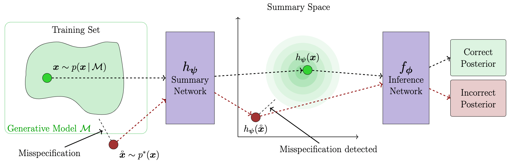
Model Misspecification

What if we are dealing with misspecified models? That is, how faithful is our amortized inference if the generative model is a poor representation of reality? A modified loss function optimizes the learned summary statistics towards a unit Gaussian and reliably detects model misspecification during inference time.

In order to use this method, you should only provide the summary_loss_fun argument to the AmortizedPosterior instance:

amortized_posterior = bf.amortizers.AmortizedPosterior(inference_net, summary_net, summary_loss_fun='MMD')

The amortizer knows how to combine its losses and you can inspect the summary space for outliers during inference.

References and Further Reading

• Schmitt, M., Bürkner P. C., Köthe U., & Radev S. T. (2022). Detecting Model Misspecification in Amortized Bayesian Inference with Neural Networks. ArXiv preprint, available for free at: https://arxiv.org/abs/2112.08866

Model Comparison

BayesFlow can not only be used for parameter estimation, but also to perform approximate Bayesian model comparison via posterior model probabilities or Bayes factors. Let's extend the minimal example from before with a second model $M_2$ that we want to compare with our original model $M_1$:

def simulator(theta, n_obs=50, scale=1.0):
    return np.random.default_rng().normal(loc=theta, scale=scale, size=(n_obs, theta.shape[0]))

def prior_m1(D=2, mu=0., sigma=1.0):
    return np.random.default_rng().normal(loc=mu, scale=sigma, size=D)

def prior_m2(D=2, mu=2., sigma=1.0):
    return np.random.default_rng().normal(loc=mu, scale=sigma, size=D)

For the purpose of this illustration, the two toy models only differ with respect to their prior specification ($M_1: \mu = 0, M_2: \mu = 2$). We create both models as before and use a MultiGenerativeModel wrapper to combine them in a meta_model:

model_m1 = bf.simulation.GenerativeModel(prior_m1, simulator, simulator_is_batched=False)
model_m2 = bf.simulation.GenerativeModel(prior_m2, simulator, simulator_is_batched=False)
meta_model = bf.simulation.MultiGenerativeModel([model_m1, model_m2])

Next, we construct our neural network with a PMPNetwork for approximating posterior model probabilities:

summary_net = bf.networks.SetTransformer(input_dim=2)
probability_net = bf.networks.PMPNetwork(num_models=2)
amortized_bmc = bf.amortizers.AmortizedModelComparison(probability_net, summary_net)

We combine all previous steps with a Trainer instance and train the neural approximator:

trainer = bf.trainers.Trainer(amortizer=amortized_bmc, generative_model=meta_model)
losses = trainer.train_online(epochs=3, iterations_per_epoch=100, batch_size=32)

Let's simulate data sets from our models to check our networks' performance:

sims = trainer.configurator(meta_model(5000))

When feeding the data to our trained network, we almost immediately obtain posterior model probabilities for each of the 5000 data sets:

model_probs = amortized_bmc.posterior_probs(sims)

How good are these predicted probabilities in the closed world? We can have a look at the calibration:

cal_curves = bf.diagnostics.plot_calibration_curves(sims["model_indices"], model_probs)

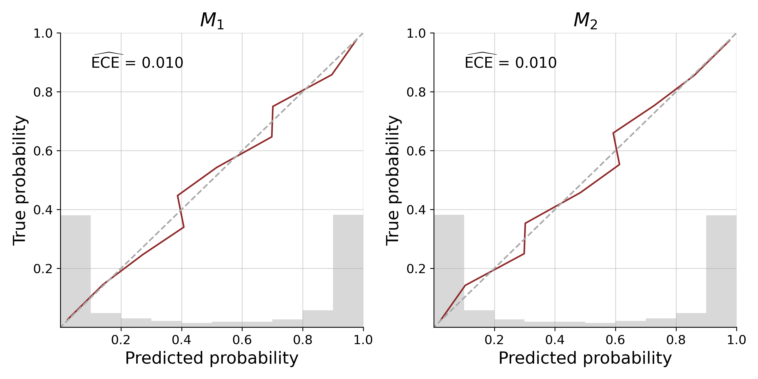
Our approximator shows excellent calibration, with the calibration curve being closely aligned to the diagonal, an expected calibration error (ECE) near 0 and most predicted probabilities being certain of the model underlying a data set. We can further assess patterns of misclassification with a confusion matrix:

conf_matrix = bf.diagnostics.plot_confusion_matrix(sims["model_indices"], model_probs)

For the vast majority of simulated data sets, the "true" data-generating model is correctly identified. With these diagnostic results backing us up, we can proceed and apply our trained network to empirical data.

BayesFlow is also able to conduct model comparison for hierarchical models. See this tutorial notebook for an introduction to the associated workflow.

References and Further Reading

• Radev S. T., D’Alessandro M., Mertens U. K., Voss A., Köthe U., & Bürkner P. C. (2021). Amortized Bayesian Model Comparison with Evidental Deep Learning. IEEE Transactions on Neural Networks and Learning Systems. doi:10.1109/TNNLS.2021.3124052 available for free at: https://arxiv.org/abs/2004.10629

• Schmitt, M., Radev, S. T., & Bürkner, P. C. (2022). Meta-Uncertainty in Bayesian Model Comparison. In International Conference on Artificial Intelligence and Statistics, 11-29, PMLR, available for free at: https://arxiv.org/abs/2210.07278

• Elsemüller, L., Schnuerch, M., Bürkner, P. C., & Radev, S. T. (2023). A Deep Learning Method for Comparing Bayesian Hierarchical Models. ArXiv preprint, available for free at: https://arxiv.org/abs/2301.11873

Likelihood Emulation

In order to learn the exchangeable (i.e., permutation invariant) likelihood from the minimal example instead of the posterior, you may use the AmortizedLikelihood wrapper:

likelihood_net = bf.networks.InvertibleNetwork(num_params=2)
amortized_likelihood = bf.amortizers.AmortizedLikelihood(likelihood_net)

This wrapper can interact with a Trainer instance in the same way as the AmortizedPosterior. Finally, you can also learn the likelihood and the posterior simultaneously by using the AmortizedPosteriorLikelihood wrapper and choosing your preferred training scheme:

joint_amortizer = bf.amortizers.AmortizedPosteriorLikelihood(amortized_posterior, amortized_likelihood)

Learning both densities enables us to approximate marginal likelihoods or perform approximate leave-one-out cross-validation (LOO-CV) for prior or posterior predictive model comparison, respectively.

References and Further Reading

Radev, S. T., Schmitt, M., Pratz, V., Picchini, U., Köthe, U., & Bürkner, P.-C. (2023). JANA: Jointly amortized neural approximation of complex Bayesian models. Proceedings of the Thirty-Ninth Conference on Uncertainty in Artificial Intelligence, 216, 1695-1706. (arXiv)(PMLR)

Support

This project is currently managed by researchers from Rensselaer Polytechnic Institute, TU Dortmund University, and Heidelberg University. It is partially funded by the Deutsche Forschungsgemeinschaft (DFG, German Research Foundation, Project 528702768). The project is further supported by Germany's Excellence Strategy -- EXC-2075 - 390740016 (Stuttgart Cluster of Excellence SimTech) and EXC-2181 - 390900948 (Heidelberg Cluster of Excellence STRUCTURES), as well as the Informatics for Life initiative funded by the Klaus Tschira Foundation.

Citing BayesFlow

You can cite BayesFlow along the lines of:

• We approximated the posterior with neural posterior estimation and learned summary statistics (NPE; Radev et al., 2020), as implemented in the BayesFlow software for amortized Bayesian workflows (Radev et al., 2023a).
• We approximated the likelihood with neural likelihood estimation (NLE; Papamakarios et al., 2019) without hand-crafted summary statistics, as implemented in the BayesFlow software for amortized Bayesian workflows (Radev et al., 2023b).
• We performed simultaneous posterior and likelihood estimation with jointly amortized neural approximation (JANA; Radev et al., 2023a), as implemented in the BayesFlow software for amortized Bayesian workflows (Radev et al., 2023b).

1. Radev, S. T., Schmitt, M., Schumacher, L., Elsemüller, L., Pratz, V., Schälte, Y., Köthe, U., & Bürkner, P.-C. (2023a). BayesFlow: Amortized Bayesian workflows with neural networks. The Journal of Open Source Software, 8(89), 5702.(arXiv)(JOSS)
2. Radev, S. T., Mertens, U. K., Voss, A., Ardizzone, L., Köthe, U. (2020). BayesFlow: Learning complex stochastic models with invertible neural networks. IEEE Transactions on Neural Networks and Learning Systems, 33(4), 1452-1466. (arXiv)(IEEE TNNLS)
3. Radev, S. T., Schmitt, M., Pratz, V., Picchini, U., Köthe, U., & Bürkner, P.-C. (2023b). JANA: Jointly amortized neural approximation of complex Bayesian models. Proceedings of the Thirty-Ninth Conference on Uncertainty in Artificial Intelligence, 216, 1695-1706. (arXiv)(PMLR)

BibTeX:

@article{bayesflow_2023_software,
  title = {{BayesFlow}: Amortized {B}ayesian workflows with neural networks},
  author = {Radev, Stefan T. and Schmitt, Marvin and Schumacher, Lukas and Elsemüller, Lasse and Pratz, Valentin and Schälte, Yannik and Köthe, Ullrich and Bürkner, Paul-Christian},
  journal = {Journal of Open Source Software},
  volume = {8},
  number = {89},
  pages = {5702},
  year = {2023}
}

@article{bayesflow_2020_original,
  title = {{BayesFlow}: Learning complex stochastic models with invertible neural networks},
  author = {Radev, Stefan T. and Mertens, Ulf K. and Voss, Andreas and Ardizzone, Lynton and K{\"o}the, Ullrich},
  journal = {IEEE transactions on neural networks and learning systems},
  volume = {33},
  number = {4},
  pages = {1452--1466},
  year = {2020}
}

@inproceedings{bayesflow_2023_jana,
  title = {{JANA}: Jointly amortized neural approximation of complex {B}ayesian models},
  author = {Radev, Stefan T. and Schmitt, Marvin and Pratz, Valentin and Picchini, Umberto and K\"othe, Ullrich and B\"urkner, Paul-Christian},
  booktitle = {Proceedings of the Thirty-Ninth Conference on Uncertainty in Artificial Intelligence},
  pages = {1695--1706},
  year = {2023},
  volume = {216},
  series = {Proceedings of Machine Learning Research},
  publisher = {PMLR}
}