Portrait Segmentation Save
Real-time portrait segmentation for mobile devices
Portrait-Segmentation
Real-time Automatic Deep Matting For Mobile Devices
Portrait segmentation refers to the process of segmenting a person in an image from its background. Here we use the concept of semantic segmentation to predict the label of every pixel (dense prediction) in an image. This technique is widely used in computer vision applications like background replacement and background blurring on mobile devices.
Here we limit ourselves to binary classes (person or background) and use only plain portrait-selfie images for matting. We experimented with the following architectures for implementing a real-time portrait segmentation model for mobile devices.
- Mobile-Unet
- DeeplabV3+
- Prisma-Net
- Portrait-Net
- Slim-Net
- SINet
The models were trained with standard(and custom) portrait datasets and their performance was compared with the help of standard evaluation metrics and benchmarking tools. Finally, the models were deployed on edge devices, using popular embedded(mobile) machine-learning platforms for real-time inference.
Dependencies
- Tensorflow(>=1.14.0), Python 3
- Keras(>=2.2.4), Kito, Scipy, Dlib
- Opencv(>=3.4), PIL, Matplotlib
pip uninstall -y tensorflow
pip install -U tf-nightly
pip install keras
pip install kito
Prerequisites
- Download training data-set
- GPU with CUDA support
- Download caffe harmonization model
- Download portrait dataset: AISegment
Datasets
The dataset consists of 18698 human portrait images of size 128x128 in RGB format, along with their masks(ALPHA). Here we augment the PFCN dataset with (handpicked) portrait images form supervisely dataset. Additionaly, we download random selfie images from web and generate their masks using state-of-the-art deeplab-xception model for semantic segmentation.
Now to increase the size of dataset and model robustness, we perform augmentation like cropping, brightness alteration, flipping, curve filters, motion blur etc.. Since most of our images contain plain background, we create new synthetic images using random backgrounds (natural) using the default dataset, with the help of a python script.
Besides the aforesaid augmentation techniques, we normalize(also standardize) the images and perform run-time augmentations like flip, shift and zoom using keras data generator and preprocessing module.
AISegment: It is a human matting dataset for binary segmentation of humans and their background. This dataset is currently the largest portrait matting dataset, containing 34,427 images and corresponding matting results. The data set was marked by the high quality of Beijing Play Star Convergence Technology Co., Ltd., and the portrait soft segmentation model trained using this data set has been commercialized.
Dataset Links:-
Also checkout the datset: UCF Selfie
Annotation Tools
A good dataset is always the first step for coming up with a robust and and accurate model, especially in the case of semantic segmentation. There are many standard datsets available for portrait(or person) segmentation like PFCN, MSCOCO Person, PascalVOV Person, Supervisely etc. But it seems that either the quality or quantity of the images are still insufficient for our use case. So, it would be a good idea to collect custom images for our training process. It is easy to collect images and create ground truth for tasks like classification or object detection; but for semantic segmentation we need to be extra-careful regarding the quality of masks. Also, data collection and annotation takes a lot of time and effort, compared to other computer vision tasks.
Here are some tools for annotation and data collection which i found to be useful in this regard:-
- Offline Image Editors - Pros: Free, High Accuracy; Cons: Manual Annotation Time; Eg: GIMP, Photoshop etc.
- Pretrained Models: Pros - Fast, Easy to Use; Cons: Limited Accuracy; Eg: Deeplab Xception, MaskRCNN etc.
- Online Annotation Tools - Pros: Automated, Easy to Use, Flexible; Cons: Price; Eg: Supervisely, Remove.bg.
- Crowd Sourcing Tools - Pros: Potential Size and Variety, Less Effort; Cons: Time, Quality; Eg: Amazon MTurk.
If you are planning to use the model on mobile phones specifically for portrait selfies, it would be a good idea to include lots of such portrait images captured using mobile phones in your dataset.
The following are some examples of the tools/models which offers reasonable accuracy and flexibility.
- unscreen.com: An automatic online tool for removing backgrounds from videos(paid).
- MODNet : A real-time portrait video matting model with very high accuracy(open-source).
Mobile-Unet Architecture
Here we use Mobilent v2 with depth multiplier 0.5 as encoder (feature extractor).
For the decoder part, we have two variants. You can use a upsampling block with either Transpose Convolution or Upsample2D+Convolution. In the former case we use a stride of 2, whereas in the later we use resize bilinear for upsampling, along with Conv2d. Ensure proper skip connections between encoder and decoder parts for better results.
Additionaly, we use dropout regularization to prevent overfitting.It also helps our network to learn more robust features during training.
Here is the snapshot of the upsampled version of model.

The other two architectures that we've experimented include mobilenet_v3 and prisma-net ,and their block diagrams are provided in the pictures directory.
How to run
Download the dataset from the above link and put them in data folder. After ensuring the data files are stored in the desired directorires, run the scripts in the following order.
1.  python train.py # Train the model on data-set
2.  python eval.py checkpoints/up_super_model-102-0.06.hdf5 # Evaluate the model on test-set
3.  python export.py checkpoints/up_super_model-102-0.06.hdf5 # Export the model for deployment
4.  python test.py test/four.jpeg # Test the model on a single image
5.  python webcam.py test/beach.jpg # Run the model on webcam feed
6.  python tflite_webcam.py  # Run the model using tflite interpreter
7.  python segvideo.py test/sunset.jpg # Apply blending filters on video
8.  python bgsub.py # Perform static background subtraction
9.  python portrait_video.py # Use portrait-net for video segmentation
10. python3 tftrt_convert.py # Convert keras model to tf-trt format
11. python3 tftrt_infer.py test/beach.jpg # Perform inference on jetson tx2
You may also run the Jupyter Notebook (ipynb) in google colaboratory, after downloading the training dataset.
In case you want to train with a custom dataset, check out the scripts in utils directory for data preparation.
Training graphs
Since we are using a pretrained mobilentv2 as encoder for a head start, the training quickly converges to 90% accuracy within first couple of epochs. Also, here we use a flexible learning rate schedule (ReduceLROnPlateau) for training the model.
Training Loss

Training Accuracy

Validation Loss

Validation Accuracy

Learning Rate Schedule

Demo
Result
1. Model Type - 1
Here the inputs and outputs are images of size 128x128.The backbone is mobilenetv2 with depth multiplier 0.5. The first row represents the input and the second row shows the corresponding cropped image obtained by cropping the input image with the mask output of the model.

Accuracy: 96%, FPS: 10-15
2. Model Type - 2
Here the inputs and outputs are images of size 224x224. The backbone is mobilenetv3 with depth multiplier 1.0. The first row represents the input and the second row shows the corresponding cropped image obtained by cropping the input image with the mask output of the model.

Accuracy: 97%, FPS: 10-15
3. Model Type - 3
Here the inputs and outputs are images of size 256x256. The prisma-net architecture is based on unet and uses residual blocks with depthwise separable convolutions instead of regular convolutional blocks(Conv+BN+Relu). Also,it uses elementwise addition instead of feature concatenation in the decoder part.
The first row represents the input and the second row shows the corresponding cropped image obtained by cropping the input image with the mask output of the model.

Accuracy: 96%, FPS: 8-10
NB: Accuracy measured on a predefined test data-set and FPS on the android application, using Oneplus3.
Failure cases

When there are objects like clothes, bags etc. in the background the model fails to segment them properly as background, especially if they seem connected to the foreground person. Also if there are variations in lighting or illumination within the image, there seems to be a flickering effect on the video resulting in holes in the foreground object.
Portrait-net
The decoder module consists of refined residual block with depthwise convolution and up-sampling blocks with transpose convolution. Also,it uses elementwise addition instead of feature concatenation in the decoder part. The encoder of the model is mobilnetev2 and it uses a four channel input, unlike the ohter models, for leveraging temporal consistency. As a result, the output video segmentaion appears more stabilized compared to other models. Also, it was observed that depthwise convolution and elementwise addition in decoder greatly improves the speed of the model.
Here is the model summary:-
1. Model 1
- Dataset: Portrait-mix (PFCN+Baidu+Supervisely)
- Device: Oneplus3 (GPU: Adreno 530)
- Size: 224x224
| Metrics | Values |
|---|---|
| mIOU | 94% |
| Time | 33ms |
| Size | 8.3 MB |
| Params | 2.1M |
2. Model 2
- Dataset: AISegment
- Device: Redmi Note 8 Pro (GPU: Mali-G76 MC4)
- Size: 256x256
| Metrics | Values |
|---|---|
| mIOU | 98% |
| Time | 37ms |
| Size | 8.3 MB |
| Params | 2.1M |
NB: Accuracy measured on a random test data-set and executiom time(GPU) using tflite benchmark tool.
Deeplab, Quantization Aware Training and ML Accelerators
DeepLab is a state-of-art deep learning model for semantic image segmentation. It was originally used in google pixel phones for implementing the portrait mode in their cameras. Later, it was shown to produce great results with popular segmentation datsets like pascal voc, cityscapes, ADE20K etc. Here, we use a deeplab model with mobilenetv2 as backbone for portrait segmentation. The deeplabv3+ model uses features like depthwise convolution, atrous convolution(dilated) and relu6 activation function, for fast and accurate segmentation. Here, we do not use ASPP blocks for training, for the sake of higher inference speeds. The model is trained with output stride 16 and exported for inference with output stride of 8.
Initially, we need to train a non-quantized model with AISegment dataset until convergence. For this purpose, we use a pretrained deeplab model trained on coco and pascal voc with mobilenetv2 backbone and depth multiplier 0.5. For the initial checkpoint, the number of classes was 21 and input size was 513x513. We may reuse all the layer weights from the pretrained model for finetuning; except the logits. In the official training script, re-configure the settings for dataset(AISegment), final logits layer, number of classes(2) and initial checkpoint(dm 0.5). Once the model is completely trained, fine-tune this float model with quantization using a small learning rate. Finally, convert this model to tflite format for inference on android.
The quantized models can be run on android phone using it's CPU; whereas GPU typically reguires a float model. It was found that the float model on gpu and quantized model on cpu (4 threads) took about the same time for inference. Even though the quantized model seems to suffer from small accuracy loss, there were no visible differences on inference. On the other hand, gpu consumes less power than cpu for the same task. If the inference is carried out using gpu rather than cpu asynchronously, the cpu can run other operations in parallel, for maximizig the overall throughput.

A third alternative is to offload the computations to specialized devices like DSP or NPU's. These chips like the Hexagon 685 DSP(Redmi Note 7 Pro), which are sometimes referred to as “neural processing units”, “neural engines”, or “machine learning cores”, are tailored specifically to AI algorithms’ mathematical needs. They’re much more rigid in design than a traditional CPUs, and contain special instructions and arrangements (HVX architecture, Tensor Cores etc.) that accelerate certain scalar and vector operations, which become noticeable in large-scale implementations. They consume less power than CPU's or GPU's and usually runs models in FP16 or UINT8 format in a faster and efficient manner. In android we can run the quantized models on DSP using NNAPI delegate or Hexagon Delegate. The hexagon delegate leverages the Qualcomm Hexagon library to execute quantized kernels on the DSP.The delegate is intended to complement NNAPI functionality, particularly for devices where NNAPI DSP acceleration is unavailable.
Here are the benchmark results:-
Deeplab Training:-
- Tensorflow version: 1.15
- Float Train: 150k epochs,
- Quant Train: 30k
- Eval mIOU: 97%
Deeplab Testing:-
- Device: Redmi Note 7 Pro, Snapdragon 675
- Model: Deeplab_Mobilenetv2_DM05
- Input SIze: 513x513
- Output Classes: 2
| Device | Time | Mode |
|---|---|---|
| GPU: Adreno 612 | 190 ms | Float |
| CPU: Kryo 460 | 185 ms | Uint8 |
| DSP: Hexagon 685 | 80 ms | Uint8 |
The automatic mixed precision feature in TensorFlow, PyTorch and MXNet provides deep learning researcher and engineers with AI training speedups of up to 3X on NVIDIA Volta and Turing GPUs with adding just a few lines of code (Automatic Mixed Precision Training). On recent nvidia GPU's, they use tensor cores with half precision(FP16) computations to speed up the training process, while maintaining the same accuracy. Using other techniques like TensorRT and XLA we can further improve the inference speed on such devices. However, tensor cores which provide mix precision(float and int8), requires certain dimensions of tensors such as dimensions of your dense layer, number of filters in Conv layers, number of units in RNN layer to be a multiple of 8. Also, currently they support very few operations and are still in experimental stage.
Here is a bar chart comparing the INT8 performance of ML accelerators across various platforms.

SlimNet: Real-time Portrait Segmentation on High Resolution Images
Slim-net is a light weight CNN for performing real-time portrait segmentation on mobile devices, using high resolution images. We were able to achieve 99% training accuracy on the aisegment portrait dataset and run the model(1.5MB) on a mid-range android smartphone at 20 fps on deployment. Using the high resolution input images, we were able to preserve fine details and avoid sharp edges on segmentation masks, during inference .The architecture is heavily inspired from the mediapipe hair-segmentation model for android and the tflite model runs on any android device without additional API's.
The following is a brief summary of the architectural features of the model:-
-
The model is based on encoder-decoder architecture and uses PReLU activation throught the network. It hepls us to achieve faster convergence and improved accuracy.
-
The inputs are initially downsampled from a size of 512 to 128 (i,e 1/4'th). This helps us to reduce the overall computation costs; while preseving the details.
-
It uses skip connections between the encoder and decoder blocks (like unet) and helps us to extract fine details and improves gradient flow across layers.
-
Further, it uses bottleneck layers (like resnet) with depthwise convolutions for faster inference.
-
Also, it uses dilated convolution(like deeplab) and helps us to maintain larger receptive field with same computation and memory costs, while also preserving resolution.
-
Finally, the features are upsampled to full resolution(512) with the help of transposed convolutions.
Benchmark and Test Summary:-
- Dataset: AISegment
- Device: Redmi Note 8 Pro (GPU: Mali-G76 MC4)
- Size: 512x512
| Metrics | Values |
|---|---|
| Accuracy | 99% |
| Time | 50ms |
| Size | 1.5 MB |
| Params | 0.35M |
| Size | 512x512 |
The slim-net model for portrait segmentation was successfully trained using tensorflow 1.15 and exported to tflite format. The new dataset consist of 55082 images for training and 13770 images for testing. It includes portrait images fromm AISegment dataset and sythetic images with custom backgrounds. This model with input size of 512x512 took about 2 days for training on a GTX 1080 Ti with batch size of 64. Finally, a test accuracy of 99% was obtained on the test-set after 300 epochs, using a minimal learning rate of 1e^-6(after decay).

The model seems to perform well on still images; but on videos in mobile it shows some flickering effect.
SINet: Extreme Lightweight Portrait Segmentation
SINet is an lightweight portrait segmentaion dnn architecture for mobile devices. The model which contains around 86.9 K parameters is able to run at 100 FPS on iphone (input size -224) , while maintaining the accuracy under an 1% margin from the state-of-the-art portrait segmentation method. The proposed portrait segmentation model conatins two new modules for fast and accurate segmentaion viz. information blocking decoder structure and spatial squeeze modules.

-
Information Blocking Decoder: It measures the confidence in a low-resolution feature map, and blocks the influence of high-resolution feature maps in highly confident pixels. This prevents noisy information to ruin already certain areas, and allows the model to focuson regions with high uncertainty.
-
Spatial Squeeze Modules: The S2 module is an efficient multipath network for feature extraction. Existing multi-path structures deal with the various size of long-range dependencies by managing multiple receptive fields. However, this increases latency in real implementations, due to having unsuitable structure with regard to kernel launching and synchronization. To mitigate this problem, they squeeze the spatial resolution from each feature map by average pooling, and show that this is more effective than adopting multi-receptive fields.
Besides the aforementioned features, the SINet architecture uses depthwise separable convolution and PReLU actiavtion in the encoder modules. They also use Squeeze-and-Excitation (SE) blocks that adaptively recalibrates channel-wise feature responses by explicitly modelling interdependencies between channels, for improving the model accuracy. For training, they used cross entropy loss with additional boundary refinement. In general it is faster and smaller than most of the portrait segmentaion models; but in terms of accuracy it falls behind portrait-net model by a small margin. The model seems to be faster than mobilentv3 in iOS; but in android it seems likely to make only a marginal difference(due to optimized tflite swish operator).
We trained the sinet model with aisegment + baidu portrait dataset using input size 320 and cross entropy loss function, for 600 epochs and achieved an mIOU of 97.5%. The combined dataset consists of around 80K images(train+val), after data augmentaion. The final trained model has a size of 480kB and 86.91K parameters. Finally, the pytorch model was exported to ONNX and CoreML formats for mobile deployment.

In practice the model works well with simple portrait images; but for videos with more background regions the model produces artefacts on the output during inference. Unfortunaltely both the original models and aisegment retrained models suffer from this problem, even after acheiving 95% mIOU after training. In the worst case scenario, we may need to run a localizer over the image and crop out the tightly bound roi region containing person before running the segmentation model or apply morphological opening/closing over the output binary mask. But this comes with additional cost and would nullify the overall advantage of the light weight segmenation model.
Quantizing MobilenetV3 Models With Keras API
MobileNetV3 is the next generation of on-device deep vision model from google. It is twice as fast as MobileNetV2 with equivalent accuracy, and advances the state-of-the-art for mobile computer vision networks. Here we use minimalistic version of mobilenetv3 with input size 256 as the encoder part of the network. In the decoder module we use transition blocks along with upsampling layers , similar to the decoder modules in the portrait-net architecture. There are two branches in this block: one branch contains two depthwise separable convolutions and the other contains a single 1×1 convolution to adjust the number of channels. For upsampling we use bilinear resize along with the transition blocks in the decoder module. In the case of skip connections between encoder anmd decoder, we use element-wise addition instead of concatenation for faster inference speed.
During training, initially we freeze all the layers of encoder and train it for 10 epochs. After that, we unfreeze all the layers and train the model for additional 10 epochs. Finally, we perform quantization aware training on the float model, and convert all of the the models to tflite format.
Observations:-
- Using the pretrained mobilnetv3 as the encoder during training greatly improved the convergence speed. Also, the input images were normalized to [-1.0, 1.0] range before passing to the model. The float model convegerd to 98% validation accuracy within first 20 epochs.
- Using the latest tensorflow built from source and aisegment dataset with 68852 images, the training process took about 2 hours for completing 20 epochs, on a Tesla P100 GPU in google colaboratory.
- In the current tensorflow 2.3 and tf model optimization library, some layers like Rescale, Upsampling2D, Conv2DTranspose are not supported by the tf.keras Quantization Aware Training API's. For this purpose you have to install the latest nightly version or build the same from source. Similarly the mobilenetv3 pretrained models are only available in tf-nightly(currently).
- Using elementwise additon instead of concatenation on skip connection bewteen encoder and decoder greatly helped us to decrease the model size and improve it's inference time.
- After quantization aware training, even though the model size was reduced by 3x, there was no considerable loss in model accuracy.
- On POCO X3 android phone, the float model takes around 17ms on CPU and 9ms on it's GPU (>100 FPS), whereas the quantized model takes around 15ms on CPU (2 threads). We were unable to run the fully quantized models(UINT8) using nnapi opr hexagon delegate since some of the layers were not fully supported. However we can run them partially on such accelerators with decreased performance(comparatively).
Android Tflite Benchmark
To measure the performance of a tflite model on android devices, we can use the native binary benchmark tool. It provides a summary of average execution time and memory consumption of individual operators on the device(CPU, GPU and DSP). To benchmark the models on your own android device using a linux system, perform the following steps :-
- Install adb tool on your system.
sudo apt-get install android-tools-adb android-tools-fastboot.
- Connect your phone to system and copy the benchmark tool.
adb push benchmark_model_latest /data/local/tmp
- Make the binary executable.
adb shell chmod +x /data/local/tmp/benchmark_model
- Copy all the tflite models into the device.
adb push mnv3_post_quant.tflite /data/local/tmp
adb push mnv3_seg_float.tflite /data/local/tmp
adb push mnv3_seg_quant.tflite /data/local/tmp
- Optionally, copy all the hexagon delegate library files.
adb push libhexagon_interface.so /data/local/tmp
adb push libhexagon_nn_skel*.so /data/local/tmp
- Finally run the benchmarks on the device.
adb shell /data/local/tmp/benchmark_model_latest \
  --graph=/data/local/tmp/mnv3_seg_float.tflite \
  --num_threads=2 \
  ----enable_op_profiling=true

adb shell /data/local/tmp/benchmark_model_latest \
  --graph=/data/local/tmp/mnv3_seg_quant.tflite \
  --num_threads=2 \
  --enable_op_profiling=true

adb shell /data/local/tmp/benchmark_model_latest \
  --graph=/data/local/tmp/mnv3_seg_float.tflite \
  --use_gpu=true \
  --enable_op_profiling=true

adb shell /data/local/tmp/benchmark_model_latest \
  --graph=/data/local/tmp/mnv3_post_quant.tflite \
  --use_hexagon=true \
  --hexagon_profiling=true \
  --enable_op_profiling=true
Note: The benchmark binary and hexagon library files are stored in the directory - libraries and binaries.
Android Application
SegMe_V0
This version of android demo application uses the nightly experimental gpu delegate for on-device inferencing and GLSurfaceView for displaying the output on screen.
Real-time portrait video in android application

(Shot on OnePlus 3 😉)
SegMe_V1
The android tflite gpu inference library seems to be in active development and is being constantly updated. The recent OpenCL backed seems to have improved the overall performance of the gpu delegate. Also, they have released an android support library for basic image handling and processing. Hopefully, in the next release they might include full support for fp16 models and faster gpu io mechanisms.
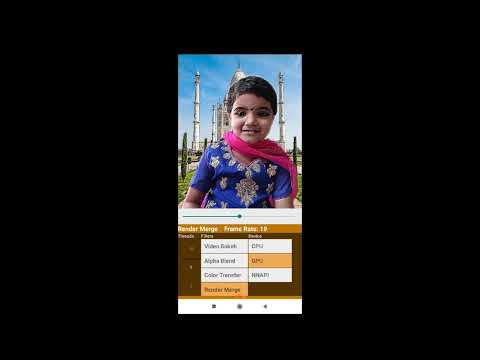
Here is a demo of android video bokeh filter ...

This version of android demo application uses the nightly experimental gpu delegate. You can directly import the gradle project using android studio and run them on you android phones. Also, ensure you have the latest updated version of android studio and gradle.
The following figure shows the overall flow of data in the demo android application.

Here, we have used image view for displaying the output for the sake of simplicity. In practice it would be a good idea to display it on a GLSurfaceview or TextureView, which are hardware accelerated. Also, the videos and textures looks better on such views(the first gif is actually a glsurface-view). Also, there is still scope for reducing the latency due to CPU-GPU data copy by directly accessing the pixel buffers from GPU, without transfering the image to CPU memory.
SegMe_V2
This version of android demo application uses the tensorflow-lite-gpu:1.15.0.The following are the additional changes and improvements from the previos version:-
- Replace imageview with gpuimageview
- Add additionals filters on video
- Improve quality of mask and video
- Add color harmonization using opencv-dnn
- Add slider control for mask thresholding
- Save the image on device
Initially, download the caffe-harmonization model and put it itn assets folder. Use single-tap on the image to change filters and long-press for saving(and harmonizing) the current frame as an image on device.
Here is a demo video of the application ...
Model running time
Summary of model size and runnig time in android
| Model Name | CPU Time (ms) | GPU Time (ms) | Parameters (M) | Size (MB) | Input Shape |
|---|---|---|---|---|---|
| deconv_fin_munet.tflite | 165 | 54 | 3.624 | 14.5 | 128 |
| bilinear_fin_munet.tflite | 542 | 115 | 3.620 | 14.5 | 128 |
| munet_mnv3_wm10.tflite | 167 | 59.5 | 2.552 | 10.2 | 224 |
| munet_mnv3_wm05.tflite | 75 | 30 | 1.192 | 4.8 | 224 |
| prisma-net.tflite | 426 | 107 | 0.923 | 3.7 | 256 |
The parameter 'wm' refers to the width multiplier (similar to depth multiplier). We can configure the number of filters of particular layers and adjust the speed-accuracy tradeoffs of the network using this paramter.
CPU Profiling :-
The benchmark tool allows us to profile the running time of each operator in CPU of the mobile device. Here is the summary of the operator profiling.
1. Deconv model
$ adb shell /data/local/tmp/benchmark_model_tf14 --graph=/data/local/tmp/deconv_fin_munet.tflite --enable_op_profiling=true --num_threads=1
Number of nodes executed: 94
============================== Summary by node type ==============================
	             [Node type]	  [count]	  [avg ms]	    [avg %]	    [cdf %]	  [mem KB]	[times called]
	          TRANSPOSE_CONV	        6	   130.565	    79.275%	    79.275%	     0.000	        6
	                     ADD	       21	    13.997	     8.499%	    87.773%	     0.000	       21
	                 CONV_2D	       34	     8.962	     5.441%	    93.215%	     0.000	       34
	                     MUL	        5	     7.022	     4.264%	    97.478%	     0.000	        5
	       DEPTHWISE_CONV_2D	       17	     3.177	     1.929%	    99.407%	     0.000	       17
	           CONCATENATION	        4	     0.635	     0.386%	    99.793%	     0.000	        4
	                     PAD	        5	     0.220	     0.134%	    99.927%	     0.000	        5
	                LOGISTIC	        1	     0.117	     0.071%	    99.998%	     0.000	        1
	                 RESHAPE	        1	     0.004	     0.002%	   100.000%	     0.000	        1

Timings (microseconds): count=50 first=164708 curr=162772 min=162419 max=167496 avg=164746 std=1434
2. Bilinear model
$ adb shell /data/local/tmp/benchmark_model_tf14 --graph=/data/local/tmp/bilinear_fin_munet.tflite --enable_op_profiling=true --num_threads=1
Number of nodes executed: 84
============================== Summary by node type ==============================
	             [Node type]	  [count]	  [avg ms]	    [avg %]	    [cdf %]	  [mem KB]	[times called]
	                 CONV_2D	       39	   534.319	    98.411%	    98.411%	     0.000	       39
	         RESIZE_BILINEAR	        5	     3.351	     0.617%	    99.028%	     0.000	        5
	       DEPTHWISE_CONV_2D	       17	     3.110	     0.573%	    99.601%	     0.000	       17
	          TRANSPOSE_CONV	        1	     0.871	     0.160%	    99.761%	     0.000	        1
	           CONCATENATION	        4	     0.763	     0.141%	    99.901%	     0.000	        4
	                     PAD	        5	     0.246	     0.045%	    99.947%	     0.000	        5
	                     ADD	       11	     0.166	     0.031%	    99.977%	     0.000	       11
	                LOGISTIC	        1	     0.119	     0.022%	    99.999%	     0.000	        1
	                 RESHAPE	        1	     0.004	     0.001%	   100.000%	     0.000	        1

Timings (microseconds): count=50 first=544544 curr=540075 min=533873 max=551555 avg=542990 std=4363
The upsamling block in the bilinear model seems to be expensive than the corresponding block in deconv model.This seems to be due to the the convolution layer using a stride of 1 with a larger image size with more channels; whereas in the case of transpose convoltuion we use a stride of 2, with lesser channels.

- Unfortunately, the benchmark tool doesn't allow gpu operator profiling.
- For the current models, it was observed that single threaded CPU execution was faster than multithreaded execution.
- Also, if you properly fuse layers like Add, Mul etc. and eliminate layers like Pad you may gain couple of milliseconds on GPU (may be more on CPU).
- We were unable to properly run the current models in NNAPI or FP16 mode due to some operator and compatibility issues.
Note: All timings measured using tflite benchmark tool on OnePlus3.
The Paradoxical GPU
Lets create some simple keras models to demonstrate and compare gpu performance with cpu ...
- Model-1
It has a convolution layer with a 3x3 identity kernel.
Model: "model_1"
_________________________________________________________________
Layer (type)                 Output Shape              Param #
=================================================================
input_1 (InputLayer)         (None, 256, 256, 1)       0
_________________________________________________________________
conv2d_1 (Conv2D)            (None, 256, 256, 1)       10
=================================================================
Total params: 10
Trainable params: 10
Non-trainable params: 0
_________________________________________________________________
- Model-2
It has one convolution layer with identity kernel and a special 1x16 kernel for data compression.
Model: "model_2"
_________________________________________________________________
Layer (type)                 Output Shape              Param #
=================================================================
input_2 (InputLayer)         (None, 256, 256, 1)       0
_________________________________________________________________
conv2d_2 (Conv2D)            (None, 256, 256, 1)       10
_________________________________________________________________
conv2d_3 (Conv2D)            (None, 256, 16, 1)        17
=================================================================
Total params: 27
Trainable params: 27
Non-trainable params: 0
_________________________________________________________________
- Model-3
It is similar to model 1; but it has four channels instead of one.
Model: "model_3"
_________________________________________________________________
Layer (type)                 Output Shape              Param #
=================================================================
input_3 (InputLayer)         (None, 256, 256, 4)       0
_________________________________________________________________
conv2d_4 (Conv2D)            (None, 256, 256, 4)       148
=================================================================
Total params: 148
Trainable params: 148
Non-trainable params: 0
- Model-4
The model is simialr to model-3. The input channels are four and we add an additional reshape layer at the end.
Model: "model_4"
_________________________________________________________________
Layer (type)                 Output Shape              Param #
=================================================================
input_4 (InputLayer)         (None, 256, 256, 4)       0
_________________________________________________________________
conv2d_5 (Conv2D)            (None, 256, 256, 1)       37
_________________________________________________________________
conv2d_6 (Conv2D)            (None, 256, 16, 1)        17
_________________________________________________________________
reshape_1 (Reshape)          (None, 256, 16)           0
=================================================================
Total params: 54
Trainable params: 54
Non-trainable params: 0
- Model-5
The model is similar to model-4. It has an additional reshape operator for resizing the flattened input tensor.
Model: "model_5"
_________________________________________________________________
Layer (type)                 Output Shape              Param #
=================================================================
input_1 (InputLayer)         (None, 196608)            0
_________________________________________________________________
reshape_1 (Reshape)          (None, 256, 256, 3)       0
_________________________________________________________________
conv2d_1 (Conv2D)            (None, 256, 256, 1)       28
_________________________________________________________________
conv2d_2 (Conv2D)            (None, 256, 16, 1)        17
_________________________________________________________________
reshape_2 (Reshape)          (None, 256, 16)           0
=================================================================
Total params: 45
Trainable params: 45
Non-trainable params: 0
- Model-6
It is similar to model-5. Here we use strided slice operator to remove the fourth channle from input instead of reshape.
Model: "model_6"
_________________________________________________________________
Layer (type)                 Output Shape              Param #
=================================================================
input_1 (InputLayer)         (None, 256, 256, 4)       0
_________________________________________________________________
lambda_1 (Lambda)            (None, 256, 256, 3)       0
_________________________________________________________________
conv2d_1 (Conv2D)            (None, 256, 256, 1)       28
_________________________________________________________________
conv2d_2 (Conv2D)            (None, 256, 16, 1)        17
_________________________________________________________________
reshape_1 (Reshape)          (None, 256, 16)           0
=================================================================
Total params: 45
Trainable params: 45
Non-trainable params: 0
- Model-7
It is similar to mode-3. Herw we use strided-slice to remove the fourth channel of input and pad operator to make the number of channels of output=4.
Model: "model_7"
_________________________________________________________________
Layer (type)                 Output Shape              Param #
=================================================================
input_1 (InputLayer)         (None, 256, 256, 4)       0
_________________________________________________________________
lambda_1 (Lambda)            (None, 256, 256, 3)       0
_________________________________________________________________
conv2d_1 (Conv2D)            (None, 256, 256, 1)       28
_________________________________________________________________
lambda_2 (Lambda)            (None, 256, 256, 4)       0
=================================================================
Total params: 28
Trainable params: 28
Non-trainable params: 0
Now, lets convert them into tflite and benchmark their performance ....
| Model Name | CPU Time (ms) | GPU Time (ms) | Parameters | Model Size (B) | Input Shape | Output Shape |
|---|---|---|---|---|---|---|
| model-1 | 3.404 | 16.5 | 10 | 772 | 1x256x256x1 | 1x256x256x1 |
| model-2 | 3.610 | 6.5 | 27 | 1204 | 1x256x256x1 | 1x256x16x1 |
| model-3 | 10.145 | 4.8 | 148 | 1320 | 1x256x256x4 | 1x256x256x4 |
| model-4 | 7.300 | 2.7 | 54 | 1552 | 1x256x256x4 | 1x256x16 |
| model-5 | 7.682 | 4.0 | 45 | 1784 | 1x196608 | 1x256x16 |
| model-6 | 7.649 | 3.0 | 45 | 1996 | 1x256x256x4 | 1x256x16 |
| model-7 | 9.283 | 5.7 | 28 | 1608 | 1x256x256x4 | 1x256x256x4 |
Clearly, the second model has one extra layer than the first model and their final output shapes differ slightly. Comparing the cpu speed of the two models, there is no surprise i.e The second model(bigger) takes slightly more time than the first.
However, if you compare the cpu performance of a model with the gpu performance, it seems counter-intutive !!!
The cpu takes less time than gpu !!!
Similarly, if you compare the gpu speed of the two models, the second one(bigger) seems to be faster than the first one, which is again contrary to our expectations !!!
So why is this happening ??? Enter the IO ...
It looks like something other than 'our model nodes' are taking up time, behind the scenes. If you closely observe, the output shape of the second model is smaller(256 vs 16). In the case of a gpu (mobile-gpu particularly), the input data is initially copied to the gpu memory from main memory (or cache) and finally after execution the result is copied back to the main memory (or cache) from the gpu memory. This copy process takes considerable amount of time and is normally proportional to data size and also depend on the hardware, copy mechanism etc. Also, for considerable speed-up the gpu should be fed with a larger model or data; otherwise the gains in terms of speed-up will be small. In the extreme cases(i.e very small inputs) the overheads will outweigh the possible benefits.
In our case, around 10ms(worst case) is taken for gpu copy or IO and this corresponds to the difference in output data size(or shape) mostly.
So, for this difference ... i.e 256x256 - 256x16 = 61440 fp32 values = 61440x4 Bytes = 245760 Bytes ~ 240KB it takes about 10ms extra copy time !!!
However, you can avoid this problem by using SSBO and and opengl, as described in the tflite-gpu documentation.
For more info refer github issue: Tensorflow lite gpu delegate inference using opengl and SSBO in android
Anyway, i haven't figure it out yet ... 😜
But wait.. what was that special filter that we mentioned perviously ??? Enter the compression ...
Let's suppose we have a binary mask as the output of the model in float32 format.i.e output of float32[1x256x256x1] type has values 0.0 or 1.0 corresponding to masked region.Now, we have a matrix(sparse) with only two values, resulting in lot of redundancies. May be we can compress them using a standard mechanisms like run length encoding(RLE) or bit packing. Considering the choices of available operators in tflite-gpu, bit packing seems to be a better alternative than RLE.
In this simple filter we perform a dot product of consecutive 16 numbers(0.0's & 1.0's) with the following filter...
[2-8, 2-7,2-6, 2-5,2-4, 2-3,2-2, 2-1,20, 21,22, 23,24, 25,26, 27]
We do this for all consecutive 16 numbers and convert each of them(group) into a sigle float32 number. We can use a convolution operation with a stride and filter of size (1,16). So, in the end we will have a output shape float32[1,256,16,1] with 16x reduced memory(copy).i.e each float32 number now represents a 16 bit binary pattern in original mask. Now the data copy time from GPU memory to cpu memory will be reduced and at the same time no information is lost due to compression.
But this method will be useful only if we can decode this data in less than 10ms(in this particular case).
Now, the third model is similar to the the first one; but it has 4 channles insted of 1.The number of paramters, size and cpu execution time of third model is greater than the first one. This is not surprising since the third model has four times the number of channels than the first one.
Now in the case of gpu, the trend is just opposite i.e gpu execution time of model-3 is less than that of model-1.This difference in number of channels alone accounts for more than 10ms time. This is beacuse of the hidden data copy happening within the gpu as mentioned in the official documentation.So, it would be a good idea to make the number of channels in layers a multiple of four throughout our model.
In model-5, we flatten the input of shape(1x256x256x3) into 1x196608, instead of adding an additional channel (i.e 4 insted of 3). But we have to include an additional rehshape operator before subsequent layers for further processing. However, it was observed that the gpu time increased considerably, even though the cpu time was almost unchanged. It looks like reshape operators takes significant amount of time in a gpu; unlike the cpu. Another strategy is to exclude the fourth channel from input using a strided slice operator as shown on model-6. This approach is slightly better than the former method of reshape operator; even though the cpu time is same for both.
Finally, we combine all the tricks and tips discussed so far in model-4. It is the largest and most complex model among the four; but it has the least gpu execution time. We have added an additional reshape layer and made the last dimension a multiple of four(i.e 16), besides the aforementioned compression technique.
These techniques have helped us to reduce the gpu execution time by 6x. Lastly, we should also note that the overall gain depends on the hardware and the model architecture.
In summary, make your data/layer size as small as possile and data/layer shape a multiple of four for improved gpu performance.Also, reduce the usage of operators that change the tensor shapes.
For more info refer code: gpucom.ipynb
-
Now according to the official tensorflow-gpu paper -On-Device Neural Net Inference with Mobile GPUs, we need to redesign our network around those 4-channel boundaries so as to avoid the redundant memory copy; but at the same time they also recommend not to use reshape operators. Now, this is huge burden put on the network designers(or application developer) part(due to limitation of opengl backend). I feel it is better to do some compile-time optimization of the model(say during conversion or internally) to avoid runtime redundant copies. But, since tflite-gpu is in it's early development stage, it's too much to ask!!!. Also, in the future we can expect the models to run faster with better hardwares(GPU,Memory etc.) and more mobile-friendly architectures.
-
Finally, if the model is very small,then we won't gain any speed-up with gpu; we can use cpu instead. Also, we cannot use a large model(say 513x513 input with 100 or more channles). It won't run due to resource constraints. Also, if it's a real-time application and you run the model continously for a long time, the device may start heating up(or slow down) and in extreme cases crashes the application.
Here is the official benchmark and comparsion of tflite models on a variety of smartphones...

To know more about the latest advances in deep learning on smartphones, checkout: AI Benchmark
Fun With Filters (Python)
Let's add some filters to harmonize our output image with the background. Our aim is to give a natural blended feel to the output image i.e the edges should look smooth and the lighting(colour) of foreground should match(or blend) with its background.
The first method is the traditional alpha blending, where the foreground images are blended with background using the blurred(gaussian) version of the mask.In the smooth-step filter, we clamp the blurred edges and apply a polynomial function to give a curved appearence to the foreground image edges.Next, we use the colour transfer algorithm to transfer the global colour to the foreground image.Also, opencv(computational photography) provides a function called seamless clone to blend an image onto a new background using an alpha mask.Finally, we use the dnn module of opencv to load a colour harmonization model(deep model) in caffe and transfer the background style to the foreground.
Here are some sample results:-

For live action, checkout the script segvideo.py to see the effects applied on a webcam video.
Also download the caffe model and put it inside models/caffe folder.
Keyboard Controls:-
Hold down the following keys for filter selection.
- C- Colour transfer
- S- Seamless clone
- M- Smooth step
- H- Colour harmonize
Move the slider to change the background image.
Tensorflowjs: Running the model on a browser
To ensure that your applications runs in a platform independent way(portabe), the easiest way is to implement them as a web-application and run it using a browser.You can easily convert the trained model to tfjs format and run them using javascript with the help of tensorflowjs conversion tools.If you are familiar with React/Vue js , you can easily incorporate the tfjs into you application and come up with a really cool AI webapp, in no time!!!
Here is the link to the portrait segmentation webapp: CVTRICKS
If you want to run it locally, start a local server using python SimpleHTTPServer. Initially configure the hostname, port and CORS permissions and then run it using your browser.
NB: The application is computaionally intensive and resource heavy.
Openvino: Deploying deep vision models at the edge
Intel's openvino toolkit allows us to convert and optimize deep neural network models trained in popular frameworks like Tensorflow, Caffe, ONNX etc. on Intel CPU's, GPU's and Vision Accelerators(VPU), for efficient inferencing at the edge. Here, we will convert and optimize a pretrained deeplab model in tensorflow using openvino toolkit, for person segmentation. As an additional step, we will see how we can send the output video to an external server using ffmpeg library and pipes.
- Download and install openvino toolkit.
- Download the tensorflow deeplabv3_pascal_voc_model, for semantic segmentation.
- Download and install ant-media server.
Once you install and configure the openvino inference engine and model optimizer, you can directly convert the tensroflow deeplab model with a single command:
python3 /opt/intel/openvino/deployment_tools/model_optimizer/mo.py --input_model frozen_inference_graph.pb --output SemanticPredictions --input ImageTensor --input_shape "(1,513,513,3)"
If the conversion is successful, two new files viz. 'frozen_inference_graph.xml' and 'frozen_inference_graph.bin' will be generated. Now, you can run the openvino python edge application for person segmentation as follows:
python3 app.py -m models/deeplabv3_mnv2_pascal_trainval/frozen_inference_graph.xml
You may view the live output rtmp stream using ant-media LiveApp in a browser or use ffplay(or vlc).
ffplay 'rtmp://localhost:1935/LiveApp/segme live=1'
The application also saves a local copy of output using OpenCV VideoWriter.
NB: Make sure that both opencv and ffmpeg are properly configured
Deploying Model on Jetson TX2 with TensorRT
Jetson TX2 is a high performance embedded AI computing device from nvidia. The module consist of six 64 bit ARM CPU's, 8 GB RAM and a 256 core Pascal GPU. The device consumes only 15W power and runs on Ubuntu 18.04. TensorRT is a C++ library that facilitates high performance inference on NVIDIA GPU's. TensorRT takes a trained network, which consists of a network definition and a set of trained parameters, and produces a highly optimized runtime engine which performs inference for that network. The library is integrated with the latest tensorflow binary(TF-TRT) and can be directly accessed via C++ or Python API.
The following are the steps to configure and run your model on jetson devices:-
- Install latest Jetpack on you device with Ubuntu 18.04.
- Install C++ version of protocol buffers library (python version has extremely long model loading time)
- Install latest tensorflow framework on your machine for jetpack 4.3.
- Convert your keras model to optimized tf-trt format using the python script (tftrt_convert).
- Run the inference code using the optimized model on webcam streams (tftrt_infer).
The inference time was reduced from 40 ms to 28 ms on using tf-trt (i.e 30% speed-up), for our prisma-net segmentation model. The new tf-trt FP16 saved model includes generic tensorflow optimizations as well as TensorRT device specific tunings. In comparsions to the original keras model, the optimized model seems to perform 10x faster inference on jetson TX2.
NB: For maximum performance, switch the power mode to MAXN(nvpmodel 0) and run the jetson_clocks script(/usr/bin) for maximum clock speed.
Mult-stream Segmentation Pipeline with Nvidia Deepstream and Jetson TX2
The deepstream sdk generic streaming analytics architecture defines an extensible video processing pipeline that can be used to perform inference, object tracking and reporting. As deepstream applications analyze each video frame, plugins extract information and store it as part of cascaded metadata records, maintaining a record's association with the source frame. The full metadata collection at the end of the pipeline represents the complete set of information extracted from the frame by deep learning models and other analytics plugins. This information can be used by the DeepStream application for display, or transmitted externally as part of a message for further analysis or long term archival. Currently, it supports applications like object detection, image classification and instance/semantic segmentation, and model formats like Caffe, Onnx and Uff for inference. Other features include plugins for IOT deployment, streaming support, multi-gpu, multi-stream and batching support for high throughput inference. These applications can be developed in C/C++ or Python and can be easily deployed on system's with a nvidia dGPU or on embedded platforms like jetson. Also, they also support FP16 and INT8 inferecne on selected hardware accelerators.
In the deepstream python application we connect two webcameras to th system(i.e. jeston dev-board) as inputs. We decode and batch the frames together with the help of various nvgst plugins and perform inference on gpu, in rela-time using nvinfer plugin. In the first application the multiple output segmentation maps are combined and displayed on screen with the help of nvsegvisual, nvegl and nvmultistreamtiler plugins; whereas in the second one, the results are streamed using rtsp streaming plugins.
Here is the schematic diagram of the segmentation pipeline (deepstream_egl_multiseg).

The above segmentation pipeline consists of the following plugins (ordered):
- GstV4l2Src - Used to capture video from v4l2 devices, like webcams and tv cards
- GstVideoConvert - Convert video frames between a great variety of video formats
- Gst-nvvideoconvert - Performs video color format conversion (I420 to RGBA)
- GstCapsFilter - Enforces limitations on data (no data modification)
- Gst-nvstreammux - Batch video streams before sending for AI inference
- Gst-nvinfer - Runs inference using TensorRT
- Gst-nvsegvisual - Visualizes segmentation results
- Gst-nvmultistreamtiler - Composites a 2D tile from batched buffers
- Gst-nvegltransform - Transform input from NVMM to EGLimage format
- Gst-nveglglessink - Render the EGL/GLES output on screen
The second streaming application (deepstream_rtsp_multiseg) includes additional plugins for rtsp streaming i.e nvv4l2h264enc, rtph264pay and udpsink.
Run the applications on jetson devices:-
- Install nvidia deepstream sdk(>=4.0) for jetson or tesla platform, pyton-gst bindings and gst-rtsp-server components by following the deepstream dev-guide documentation.
- Connect two webcams to the jetson module through USB ports.
- Run these commands on the jetson device to boost the clocks: sudo nvpmodel -m 0; sudo jetson_clocks
- Run the applications from the directory '<DeepStream 4.0 ROOT>/sources/python' (i.e python deepstream samples).
- For the streaming application, open the rtsp stream using VLC player i.e 'rtsp://{jetson-ip}:8554/ds-seg' on another system (try vlc on android).

Note: Refer onnx_nchw_conversion ipython notebooks for converting tensorflow/keras models to onnx_nchw format for deepstream inference. Also,before running the application configure the webcam properites(video source and resolution) based on your hardware settings.
Portrait Segmentaion Using Mediapipe And Slimnet
Mediapipe is an open-source framework for developing machine learning application, for mobile, desktop, web and IoT devices. It can be used to process data in various formats like images, audio and video streams. The basic idea is to construct a high-level pipeline graph for a ML workflow by integrating a set of modular components for individual operations like data transformations, model inference, I/O operations etc
Advantages:-
- Portable pipelines: The same pipeline graphs can be developed and deployed on desktops, mobile or IOT devices.
- Rapid prototyping: Most of the common image, video and ML operations can be integrated as nodes in the development workflow.
- Documentation and support: It was developed by google and has a very good documentation, with lots of demo applications.
- Extensibility: Custom operations can be easily developed in opencv(C++) and integrated into the mediapipe workflow.
Portrait segmentaion mediapipe graphs:-
The basic pipeline for video segmentaion is described in the mediapipe hair_segmentaion application. Here, we use our slimnet model on the pipeline and segment out the foreground person from the background. Additionally, we apply an edge detection filter on the masked background region of the image.

The following are the steps for building android application with bazel, mediapipe and tflite:-
- Install bazel, jdk, android sdk & ndk, and mediapipe
- Convert the slim_net model for portrait segmentaion to tflite format
- Modify the hair_segmentaion demo application from mediapipe repository
- Build the portrait_segmentaion application for android devices using bazel
- Install and run the portrait_segmentation application on mobile
Mediapipe slimnet application screenshot:-

Mediapipe portrait_segmentation(APK): slimnet android
In the android demo, we used the default mask_overlay_calculator for performing alpha blending operation. Now, if we want to perfrom some advanced blending opertations, we will have to implement it as a custom calculator in mediapipe. In this demo, we will build a portrait segmentaion aplication using custom calculators on desktop, using mediapipe. There will be two inputs: a portrait video and a background video and a single output in the form of a video file. Our aim is to blend the portrait foreground region into the background video, with the help of a segmentaion mask. As in the case of android, we will follow the basic segmentation pipeline from hair segmentaion example. Since the application uses gpu operations, choose a GPU runtime for development and deployment.
Portrait segmentation desktop:-

Segmentation via Background Subtraction: A Naive Approach
If we have a static background, we can easily obtain the mask of new objects appearing on the scene using the methods of background subtraction. Even though this seems straight-forward; there seems to be couple of challenges in this scenario. Firstly, even if objects does not move in the background, there will be small variations in corresponding pixel values due to changes in lighting, noise, camera quality etc. Secondly, if the new objects have colour similar to that of the background, it becomes difficult to find the image difference.
Here is a simple algorithm for segmentation, using background subtraction. We assume that the backgroud image or camera is static during the entire experiment.
- Capture the first 'N' background images and find the mean background image.
- Convert the background image to grayscale and apply gaussian blur.
- Capture the next frame in grayscale, with new objects and apply gaussian blur.
- Find the absolute differece between current frame and background image.
- Threshold the differecne with a value 'T' and create the binary difference-mask.
- Apply morphological operations to fill up the holes in the mask.
- Find the largest contour and remove the smaller blobs in the mask.
- Apply alpha blend on the frame with any background image, using the mask.
- Display the output on screen.
- Repeat steps 3 to 9, until a keyborad interruption.
The algorithm works pretty well, if there is proper lighting and clear colour difference between the foreground object and background. Another idea is to detect the face and exclude potential background regions based on some heuristics. Other classical methods include grabcut, active contours, feature based(HOG) detectors etc. But none of them seems to be robust, real-time and light-weight like our deep neural network models. Additionaly, using trimap-masks and depth sensors(ToF) on phone could help us acheive better visual perception and accuracy on the mobile application eg. uDepth.
Also check-out this cool application: Virtual Stage Camera
Techniques For Improving Robustness, Accuracy and Speed
Here are some advanced techniques to improve the accuracy, speed and robustness of the portrait segmentation model for videos. Most of them are inspired from the following two papers:-
- PortraitNet: Real-time portrait segmentation network for mobiledevice
- Real-time Hair Segmentation and Recoloring on Mobile GPUs
Boundary Loss: In order to improve the boundary accuracy and sharpness, we modify the last layer in the decoder module by adding a new convolution layer in parallel to generate a boundary detection map. We generate the boundary ground truth from manual labeled mask using traditional edge detection algorithm like canny or sobel, on-the-fly. Also, we need to use focal loss instead of BCE, for training the network with boundary masks. Finally, we can remove this additional convolution layer for edges and export the model for inference.
Consistency Constraint Loss: A novel method to generate soft labels using the tiny network itself with data augmentation, where we use KL divergence between the heatmap outputs of the original image and texture enhanced image, for training the model. It further improves the accuracy and robustness of the model under various lighting conditions.
Refined Decoder Module: The decoder module consists of refined residual block with depthwise convolution and up-sampling blocks with transpose convolution. Even though it includes the skip connectios similar to unet architecture, they are added to the layers in decoder module channel-wise instead of usual concatenation. Overall, this improves the execution speed of the model.
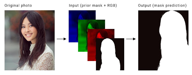
Temporal Consistency: A video model should exhibit temporal redundancy across adjacent frames. Since the neighbouring frames are similar, their corresponding segmentation masks should also be similar(ideally). Current methods that utilize LSTM, GRU(Deep) or Optical flow(Classic) to realize this are too computationally expensive for real-time applications on mobile phones. So, to leverage this temporal redundancy, we append the segmentation output of the previous frame as the fourth channel(prior) of the current input frame during inference. During training, we can apply techniques like affine transformations, thin plate spline smoothing, motion blur etc. on the annotated ground truth to use it as a previous-mask. Also, to make sure that the model robustly handles all the use cases, we must also train it using an empty previous mask.
High resolution Input: In our original pipeline, we downsample our full resolution image from mobile camera to a lower resolution(say 128 or 224) and finally after inference, we upsample the output mask to full resolution. Even though output results are satisfactory; there are couple of problems with this approach. Firstly, the resized mask edges will be coarse(stair-case) or rough and extra post-processing steps will be needed to smoothen the mask. Secondly, we loose lots of details in the input due to downsampling and thus it affects the output mask quality. If we use a larger input size, it would obviously increase the computation time of the model. The primary reason for this increase, is the increase in number of parameters. Also, on a mobile device the CPU-GPU data transfer takes considerable amount of time, especially when the inputs are large. To solve the latter problem, we can use techniques like SSBO(low level) or frameworks like mediapipe(high-level) which already comes with a optimized inference pipeline. As for the former one, we can slightly modify the architecture of the model such that, for most part convolutions happen at a lower spatial dimension. The idea is to rapidly downsample the input at the beginning of the network and work with a smaller resolution image throughout a deeper version of the network . Finally, upsample the result from the final layers to full scale, within-the model. Thus, it ensures that the model learns the upsampling or downsampling itself and eliminates the need for a separate post-inference resize or smoothing.
Advanced Activation Function: Newer activation functions like Swish(mobilenetv3) or PRelu(mediapipe hair segmentation) seems to give better accuracy with lower execution time. However, we may need to restructure our network and implement custom-layers for such operators to properly run on mobile GPU, using tensorflow-lite.
The portrait-net model for videos was successfully trained using pytorch and exported to tflite format. The new dataset consist of 60,000 images for training and 8852 images for testing.It includes portrait images from AISegment dataset and sythetic images with custom backgrounds. This model with input size of 256x256 took about 5 days for training on a GTX 1080 Ti with batch size of 48. Finally, an mIOU of 98% was obtained on the test-set after 500 epochs, using a minimal learning rate of 1e^-6(after decay). The new portrait dataset, conversion scripts, trained models and corresponding inference code in python are also available in the respective folders. It can be easily used with the current android application(SegMeV2) by slightly modifying the I/O handling steps. A frame rate of 30 FPS was acheived using this model.
Here is the link to Android application: SegVid.apk
It supports 32 and 64 bit ARM architectures(armeabi-v7a and amr64-v8a). The application works best on portrait videos with good lighting conditions.
Note: For more information on training, check out the respective papers and repositories.
Post-Training Quantization and Edge TPU Inference
Quantizing deep neural networks uses techniques that allow for reduced precision representations of weights and, optionally, activations for both storage and computation(for eg. UINT8 or FLOAT16). It can reduce model size while also improving CPU and hardware accelerator latency, with little degradation in model accuracy. Tensorflow lite supports two types of quantization viz. quantization qware training and post training quantization. Even though the former method produces better accuracy, it is only supported by a few subset of convolutional neural network architectures. Also, currently tensorflow 2.0 and keras does not support this technique. Therefore, we are left with only one option i.e Post-training quantization.
Again, there are two types of post-training quantization: weight quantization and full integer quantization(float also). In the weight quantization, only the weights are converted to 8 bit integer format. At inference, weights are converted from 8-bits of precision to floating point and computed using floating-point kernels. In full integer quantization, we use integer weights and integer computations on the model layers. For this purpose, you need to measure the dynamic range of activations and inputs by supplying a representative data set, during the conversion process. The potential advantages include faster inference, reduced memory usage and access to hardware accelerators like TPU, NPU etc. On the flip side, it can lead to accuracy degradation, especially in scenarios where high pixel accuracies or precise boundaries are desired.
The Coral USB Accelerator is a USB device that provides an Edge TPU as a coprocessor for your computer. It accelerates inferencing for your machine learning models when attached to the host computer. Initially, we need to convert our float model to a fully quantized format, using the aforementioned techniques. Then, we need to convert the quantized model to tpu format with the help of edge tpu compiler. Finally, we can run the tpu model on the device with the help of edge tpu runtime library. Compared to quantized inference on CPU, TPU offers additional advantages like faster inference, reduced power etc.
The portrait-net and prisma-net models were successfully converted to quantized format. Their size was reduced by about 3x and their outputs were verified using a test dataset. We were able to convert the prisma-net model to tpu format; but unfortunately the portrait-net model failed in the conversion process(layer compatability issue). The edge tpu model took only a mere 12.2 ms for inference, in comparison to the inference on CPU, which took about 4357.0ms with quantized model and 500ms with float model. The CPU(i7-3632QM CPU @ 2.20GHz) might mostly be using a single core for inference. But even if we include other possible overheads, this 40x speed-up seems to be worth the effort. Besides, it consumes 20 times less power than CPU.
Key Insights and Drawbacks
- Always start experimentation with standard/pretrained networks. Also try out default/standard hyperparameter settings before experimentation. Often standard datasets may not be sufficient for your particular application scenario .So, do not hesitate to re-train your model with a custom dataset specific to your application or use case (For eg:- if a model can’t handle a specific pose, it may be that the dataset is not representative enough).
- Make sure your ground truth is correct/uncorrupted and is in desired format before training (even standard dataset).Your model is only as good as your dataset. If you want very high accuracy and robustness on a mobile app, make sure you have a large dataset(10K or more)of images for training, preferably captured using a mobile device.
- For mobile devices, make sure you use a mobile-friendly architecture (like mobilenet) for training and deployment. These architectures extensively use depth-wise or separable convolutions instead of normal convolutions.
- Using google colaboratory along with google drive for training was EASY & FUN.It provides high end GPU (RAM also) for free.
- Some of the mobile optimization tools(even TF) are still experimental (GPU deegate, NNAPI, FP16 etc.) and are buggy.They support only limited operations and edge devices.
- Even state-of-the art segmenation models(deeplab-xception) seems to suffer from false positives (even at higher sizes), when we test them on a random image.
- The segmentaion maps produced at this low resolution (128x128) have coarse or sharp edges (stair-case effect), especially when we resize them to higher resolution.
- To tackle the problem of coarse edges, we apply a blur filter (also antialiasing at runtime) using opencv and perform alpha blending with the background image. Other approach was to threshold the blurred segmentation map with smooth-step function and finally mix the foreground and background with mask, using GLSL shaders or Renderscript.
- In android we can use tensorflow-lite gpu-delegate to speed up the inference.It was found that flattening the model output into a rank 1 (or 2) tensor helped us to reduce the latency due to GPU-CPU data transfer.Also this helped us to post-process the mask without looping over a multi-dimensional array.
- Using opencv (Android NEON) for post-processing helped us to improve the speed of inference.But this comes at the cost of additional memory for opencv libraray in the application.
- Still, there is a scope for improving the latency of inference by performing all the postprocessing in the GPU, without transfering the data to CPU. This can be acheived by using opengl shader storge buffers (SSBO). We can configure the GPU delegate to accept input from SSBO and also access model output from GPU memory for further processing (wihout CPU) and subsequent rendering.
- Make sure most(all if possible) of your nodes or layers have a shape of the form NHWC4 (i.e channels-C are multiple of four), if you plan to use tflite gpu delegate. This ensures that there are no redundant memory copies during shader execution. Similarly avoid reshape operators, whenever possible.These tricks can significanlty improve the overall speed or runnig time of your model on a mobile device(GPU).
- The parameters like image size, kernel size and strides (ie. of form - [x,x]) have significant impact on model running time(especially cpu). Clearly, the model layer running time seems to be proportional to the square of image and kernel size(x) and inversely proportional to the square of stride values(x),(other params. being const. in each case). This could be mostly due to the proportional increase/decreae in MAC operations.
- The difference between the input image frame rate and output mask generation frame rate may lead to an output(rendering), where the segmentation mask lags behind current frame.This stale mask phenomena arises due to the model(plus post-processing) taking more than 40ms (corr. to 25 fps input) per frame (real-time video), during an asynchronous execution. The solution is to render the output image in accordance to the mask generation fps (depends on device capability) or reduce the input frame rate.
- If your segmentaion-mask output contains minor artifacts, you can clean them up using morphological operations like opening or closing. However it can be slightly expensive if your output image size is large, especially if you perform them on every frame output.
- If the background consists of noise, clutter or objects like clothes, bags etc. the model fails miserably.
- Even though the stand-alone running time of exported (tflite) model is low(around 100 ms),other operations like pre/post-processing, data loading, data-transfer etc. consumes significant time in a mobile device.
- The models trained with resize bilinear(default parameters) in tensorflow seems to suffer from a problem of mask shifting.This problem occurs if the image size is even (i.e bilinear_128 model in our case).The pixels in the output mask seems to be sligtly shifted horizontaly in one direction(left/right).
- Opencv dnn module provides support for running models trained on popular platforms like Caffe,Tensorflow, Torch etc.It supports acceleration through OpenCL, Vulkan, Intel IE etc.It also supports variety of hardwares like CPU,GPU and VPU.Finally, we can also run smaller FP16 models for improved speed.
- Once you are familiar with tensorflow, it is fairly easy to train and perform inference using tensorflowjs.It also comes with support of WebGL backend for accelerating the inference and training process.Th main advantage is the portability of the application i.e it can be run on PC, phones or tablet without any modifications.
- The minimalistic version of mobilenetv3 with depth-multiplier 1 and input size 224 has almost the same latency as the mobilenetv2 with input size 128 and depth multiplier 0.5. The accuracy was also found to be same on the test-datastet; however the edges of the segmentation map was much smoother in mobilenetv3, with higher image size. Theoretically, it should also be able to capture more details than the smaller 128 model.
- Instead of using an explicit softmax layer as the final layer of the model during training, pushing this softmax activation into the cross-entropy loss layer(with from_logits=True) significantly simplifies the loss computation and makes it more numerically stable. In the training dataset, the input images may be encoded in jpg format for saving memory; but the segmentation masks should be saved in png format(lossless). Also during preprocessing step, ensure that you use nearest neighbour interpolation while resizing the segmentation masks(hard labels).
- A fully quantized tflite seems to be significantly slower than float32 version, while performing inference on a pc using tflite python interpreter.But for mobile CPUs, considerable speedup can be observed. On the other hand, the quantized model gives more than 10x speed-up on a edge TPU compared to the float32 model on CPU.
- Most of the standard person/portrait segmentation datasets contain lots of images different from the real world mobile phone portraits. A large number of images have plain or blurred backgrounds and most of them are captured under good/ideal lighting conditions. Even if we replace the background with image composting techniques, the resulting images looks unnatural.
- In general, trimap-free models always tend to overfit the training set and cannot generaliz well on realworld data. On the other hand trimap models which contain additional layers for techniques like boundary attention, high resolution feature fusion etc., for improving the boundary details(eg. fine hair details) have higher execution time on mobile devices.
- The original deeplab model was trained using pascal voc dataset, with white edges(similar to trimaps) around subject boundaries in labels set to be ignored class(pixels). In the original portrait-net architecture none of the convolutional layers contain a bias term.
- No amount of skillful post-processing and attempting to extract useful data from the output will make up for a poor model choice, or one where too many sacrifices were made for speed.
- Usage of strided convolution or pooling layer helps us to capture global information by enlarging receptive field size; but they can also lead to loss of detailed local information.
- Recently, many vendors like Apple, Huawei and Qualcomm have come up with their own Vision API's, NPU's, DSP's, ISP's etc. The performace of these devices seems to be on par with the high-end PC's. After model exporting, we can directly run them on high resolution images in real-time. However, many of the features are still experimental, some are not open-source and there is a lack of proper standardization among the hardware and software vendors in this domain.
TODO
- Combine all techniques and train a TF2.0 model
- Use a bigger image for training(224x224)
- Try quantization-aware training
- Train with mixed precision (FP16)
- Optimize the model by performing weight pruning
- Improve accuracy & reduce artifacts at runtime
- Leverage temporal consistency in video
- Include boundary refinement techniques
- Reduce GPU memory copy time
- Incroporate depth information
- Apply photorealistic style transfer on foreground based on background image
License
This project is licensed under the terms of the MIT license.
Versioning
Version 1.0
Authors
Anil Sathyan
Acknowledgments
- https://www.tensorflow.org/model_optimization
- https://www.tensorflow.org/lite/performance/gpu_advanced
- https://github.com/cainxx/image-segmenter-ios
- https://github.com/gallifilo/final-year-project
- https://github.com/dong-x16/PortraitNet
- https://github.com/ZHKKKe/MODNet
- https://github.com/clovaai/ext_portrait_segmentation
- https://github.com/tantara/JejuNet
- https://github.com/lizhengwei1992/mobile_phone_human_matting
- https://github.com/dailystudio/ml/tree/master/deeplab
- https://github.com/PINTO0309/TensorflowLite-UNet
- https://github.com/xiaochus/MobileNetV3
- https://github.com/yulu/GLtext
- https://github.com/berak/opencv_smallfry/blob/master/java_dnn
- https://github.com/HasnainRaz/SemSegPipeline
- https://github.com/onnx/tensorflow-onnx
- https://github.com/onnx/keras-onnx
- https://machinethink.net/blog/mobilenet-v2/
- On-Device Neural Net Inference with Mobile GPUs
- AI Benchmark: All About Deep Learning on Smartphones in 2019
- Searching for MobileNetV3
- Google AI Blog: MobilenetV3
- Youtube Stories: Mobile Real-time Video Segmentation
- Facebook SparkAR: Background Segmentation
- Learning to Predict Depth on the Pixel 3 Phones
- uDepth: Real-time 3D Depth Sensing on the Pixel 4
- iOS Video Depth Maps Tutorial
- Huawei: Portrait Segmentation
- Deeplab Image Segmentation
- Tensorflow - Image segmentation
- Official Tflite Segmentation Demo
- Tensorflowjs - Tutorials
- Hyperconnect - Tips for fast portrait segmentation
- Prismal Labs: Real-time Portrait Segmentation on Smartphones
- Keras Documentation
- Boundary-Aware Network for Fast and High-Accuracy Portrait Segmentation
- Fast Deep Matting for Portrait Animation on Mobile Phone
- Adjust Local Brightness for Image Augmentation
- Pyimagesearch - Super fast color transfer between images
- OpenCV with Python Blueprints
- Pysource - Background Subtraction
- Learn OpenCV - Seamless Cloning using OpenCV
- Deep Image Harmonization
- Tfjs Examples - Webcam Transfer Learning
- Opencv Samples: DNN-Classification
- Deep Learning In OpenCV
- BodyPix - Person Segmentation in the Browser
- High-Resolution Network for Photorealistic Style Transfer
- Tflite Benchmark Tool
- TensorFlow Lite Android Support Library
- TensorFlow Lite Hexagon delegate
- Tensorflow lite gpu delegate inference using opengl and SSBO in android
- Udacity: Intel Edge AI Fundamentals Course
- Udacity: Introduction to TensorFlow Lite
- Android: Hair Segmentation with GPU
- Image Effects for Android using OpenCV: Image Blending
- Converting Bitmap to ByteBuffer (float) in Tensorflow-lite Android
- Real-time Hair Segmentation and Recoloring on Mobile GPUs
- PortraitNet: Real-time portrait segmentation network for mobile device
- ONNX2Keras Converter
- Google: Coral AI
- Hacking Google Coral Edge TPU
- Peter Warden's Blog: How to Quantize Neural Networks with TensorFlow
- Tensorflow: Post Training Quantization
- Qualcomm Hexagon 685 DSP is a Boon for Machine Learning
- How Qualcomm Brought Tremendous Improvements in AI Performance to the Snapdragon 865
- TF-TRT 2.0 Workflow With A SavedModel
- NVIDIA-AI-IOT: Deepstream_Python_Applications
- Awesome Tflite: Models, Samples, Tutorials, Tools & Learning Resources.
- Google: Machine Learning Bootcamp for Mobile Developers
- Machinethink: New mobile neural network architectures
- Deeplab Tflite Tfhub
- MediaPipe with Custom tflite Model
- Google Mediapipe Github
