Lightvector GoNN Save
Sandbox for playing with neural nets for Go
Go Neural Net Sandbox
See here for a fully-working Alpha-Zero-like self-training loop that is a major continuation of the research and experimentation in this repo: https://github.com/lightvector/KataGo.
This repo was a sandbox for personal experimentation in Go neural net training and Go AI. Further work and research has since moved to a new repo KataGo, and this repo has been left here primarily as a showcase of earlier experiments and results. The code should still work though (at least with older versions of Tensorflow), so if you're interested in experimenting with neural nets and supervised learning on human Go games, see below for how to get started.
See LICENSE for software license. License aside, informally, if do you successfully use any of the code or any wacky ideas about neural net structure explored in this repo in your own neural nets or to run any of your own experiments, I would to love hear about it and/or might also appreciate a casual acknowledgement where appropriate. Yay.
To experiment with pre-trained neural nets alone:
- You must have Python3 and Tensorflow installed.
- Either download a pre-trained model (https://github.com/lightvector/GoNN/releases) or train one yourself (see below).
- Do things with the trained model
- Run a GTP engine using the model to make moves directly:
./play.py -model <MODELS_DIRECTORY>/model<EPOCH> - Dump one of the raw weight matrices:
./visualize.py -model-file <MODELS_DIRECTORY>/model<EPOCH> -dump p2/w:0 - Directly run a model on a position from an sgf file:
./eval_sgf.py -model-file <MODELS_DIRECTORY>/model<EPOCH> -sgf SGFFILE -move TURNNUMBER
- Run a GTP engine using the model to make moves directly:
Training a neural net:
If you'd like to train your own neural net model and/or experiment with the architectures in this repo, here are the steps.
- You must have CMake installed with a minimum version of 3.8.2 (https://cmake.org/download/)
- You must have HDF5 installed for C++ (https://support.hdfgroup.org/HDF5/release/obtainsrc.html).
- Training consists of converting .sgf files into training rows written in HDF5 format, then reading that HDF5 file in Python to train using numpy and h5py to feed them to Tensorflow.
- The utility that converts .sgf to .h5 is written in C++. Compile it using CMake and make in the cpp directory, which expects you to have h5c++ available:
-
cd cpp -
cmake . -DBUILD_WRITE=1 -
make
-
- Run the compiled
writeexecutable with appropriate flags on a directory of SGF files to generate an h5 file of preprocessed training data.- Example:
./write -pool-size 50000 -train-shards 10 -val-game-prob 0.05 -gamesdir <DIRECTORY WITH SGF FILES> -output <TARGET>.h5- writes an h5 file making 10 passes over the games with a running buffer of 50000 rows to randomize the order of outputted rows, reserving 5% of games as a validation set.
- Example:
- Back up in the root directory, run train.py using that h5 file to train the neural net.
- Example:
./train.py -traindir <DIRECTORY TO OUTPUT MODELS AND LOGS> -gamesh5 <H5FILE>.h5 - By default, it considers 1 million samples to be one epoch. If you want to see initial results more quickly you can pass
-fast-factor Nto divide this and a few other things by N, and-validation-prop Pto only use P proportion of the validation set, but you will probably want to manually modify train.py (seeTRAINING PARAMETERSsection) as well as model.py (to try a much smaller neural net first). - Depending on how much training data you have and how long you're willing to train for, you probably want to edit the
knotsin train.py that determine the learning rate schedule. - If you getting errors due to running out of GPU memory, you probably want to also edit train.py to shrink the
batch_sizeand/or thevalidation_batch_size.
- Example:
Running a full-fledged Go engine:
There is an implementation of MCTS in this repo along with a GTP engine and an simple SGF command-line analyis tool backed by the MCTS engine. If you'd like to use a model you've trained or a pre-trained model with this MCTS implementation, you can try these steps.
- You must have CMake installed with a minimum version of 3.8.2 (https://cmake.org/download/)
- You must have either ONE of these:
- CUDA 9.0 and CUDNN 7.0 installed (https://developer.nvidia.com/cuda-toolkit) (https://developer.nvidia.com/cudnn) and a GPU capable of supporting them. I'm unsure how version compatibility works with CUDA, there's a good chance that later versions than these work just as well, but I have not personally upgraded yet.
- Tensorflow compiled and installed as a shared library. Official support for this appears to be a bit lacking, and building against Tensorflow normally requiries installing Bazel and building code jointly with the Tensorflow source with their build system. To build instead as a linkable shared library, I have successfully used https://github.com/FloopCZ/tensorflow_cc at one point, prior to switching to directly using CUDA. But it was not easy, so I recommend CUDA assuming you have an appropriate nvidia GPU.
- The code written in C++. Compile it using CMake and make in the cpp directory:
-
cd cpp -
cmake . -DBUILD_MCTS=1 -DUSE_CUDA_BACKEND=1ORcmake . -DBUILD_MCTS=1 -DUSE_TENSORFLOW_BACKEND=1depending on which one you're using -
make
-
- Run the compiled
mainexecutable to do various things. Edit the configs to change parameters as desired.- Example:
./main gtp -nn-model-file <FILE> -config-file configs/gtp_example.cfg- Run a simple GTP engine using a given neural net and example provided config. - Example:
./main evalSgf -nn-model-file <FILE> -sgf-file <SGF>.sgf -move-num <MOVENUM> -config-file configs/eval_sgf.cfg- Have the bot analyze the specified move of the specified SGF.
- Example:
Experimental Notes
You can see the implementations of the relevant neural net structures in "model.py", although I may adapt and change them as time goes on.
History
- Oct-Dec 2018 - Busy working the last few months on infrastructure to test a variety of experimental ideas for AlphaGoZero-like training, hope to have things to report soon. In the meantime, a few more updates: Global pooling boosts playing strength. Dilated convolutions not so exciting for playing strength. MCTS can maybe be improved by making it more minimax-like. A brief note about cPUCT scaling. Also discovered that due to a bug, most earlier results that reported a number of visits were actually performed with that many playouts (i.e. in addition to tree reuse from previous moves) - corrected the appropriate sections.
- Sept 2018 - (forgot to include in the previous update) update about parametric relus and the value head.
- July-Aug 2018 - Implemented a full Go bot from the ground up with multithreaded MCTS with batched NN evaluations, and the groundwork for supporting a variety of rulesets in the future. Began experimenting with search in addition to neural net training. Tested strength of cross-entropy vs L2 value nets, experimented with first-play-urgency, and experimented with the cpuct exploration parameter.
- May-June 2018 - No significant architectural changes, but added player ranks as an input feature to the neural net and included a lot of amateur games in the training set. Filtered pro games with the resulting net to find instructive positions for players of different ranks, producing a neat collection of Go problems: neuralnetgoproblems.com. Cleaned up a few input features and tried a slightly larger net with more training.
- Apr 2018 - Added a row to the current results reflecting the large improvement from embedding global pooled properties in the middle of the neural net rather than only the policy head, along with some minor adjustments to learning rates and other tweaks.
- Mar 2018 - Much larger neural nets and updates to current results. Global pooled properties are good in the main trunk of the resnet as well! Also, increasing center-position learning rates everywhere else in the net helps training speed a little. Promising experiments with dilated convolutions, and a note about making neural nets not always need history.
- Feb 2018 - Tried special ladder blocks in the policy, tried ladders as a training target, retested global pooled properties. And ran new experiments with net architecture - wide low-rank residual blocks, parametric ReLUs, chain pooling, and some observations on redundancy in models
- Dec 2017 - Initial results and experiments - special ladder residual blocks, global pooled properties
Raw Neural Net Results
As of the end of April 2018, the best neural nets I've been training from this sandbox have been quite good at matching or exceeding results I've seen published elsewhere in a head-to-head comparison of the neural nets' raw accuracy stats, presumably due to the combination of the various enhancements discussed below. See this table for a summary of results (bolded) in comparison with other published results:
| Neural Net | Structure | Params | KGS Top1 | GoGoD Top1 | Training Steps | Vs GnuGo | Vs Pachi |
|---|---|---|---|---|---|---|---|
| Clark and Stokey (2015) | CNN 8xVarious | ~560,000 | 44.4% | 41.1% | 147M | 87% (172/200) | |
| Maddison et al. (2015) | CNN 12x(64-192) | ~2,300,000 | 55.2% | 685M x 50 + 82M | 97% (/300?) | 11% (/220?) | |
| AlphaGoFan192 (2016) | CNN 13x192 | 3,880,489 | 55.4% | 340M x 50 | 85% (w/RL) | ||
| AlphaGoFan256 (2016) | CNN 13x256 | 6,795,881 | 55.9% | ||||
| This Sandbox (Mar 2018) | ResNet 5x192 | 3,597,792 | 56.8% | 52.5% | 205-209M | 99.2% (496/500) | |
| Darkforest (2016) | CNN 12x384 | 12,329,756 | 57.1% | 128M | 100% (300/300) | 72.6% (218/300) | |
| Cazenave (2017) | ResNet 10x256 | 12,098,304 | 58.2% | 54.1% | 380M | ||
| This Sandbox (Mar 2018) | ResNet 12x192 | 8,250,720 | 58.2% | 54.2% | 325-333M | 100% (500/500) | 90.0% (45/50) |
| Cazenave (2017) | ResNet 14x256 | 16,816,896 | 54.6% | 355M | |||
| This Sandbox (Apr 2018) | ResNet 12x192 | 8,057,424 | 58.6% | 54.7% | 201M-209M | ||
| This Sandbox (Jun 2018) | ResNet 12x224 | 10,950,416 | 55.3% | 301M | |||
| AlphaGoZero(2017) | ResNet 20x256 | 22,837,864 | 60.4% | >1000M? |
As seen in the above table, thanks to the various enhancements I've been playing with, the neural nets in this sandbox compare quite favorably, matching or surpassing accuracy results for neural nets with larger numbers of parameters. They require fewer training steps to achieve these results and are probably computationally faster to evaluate per step (I currently don't use any techniques such as rotational equivariance or other weight representations that reduce the number of parameters in a way that doesn't also reduce the computation cost).
However, one thing to keep in mind is that not all of the results in this table are precisely comparable. In the above papers, different authors often made different choices about the date range, what range of player ranks to allow, what version of the dataset to use (GoGoD has biannual updates), and whether to include or exclude handicap games. Overall, I think most of these choices shouldn't affect the results too much, but I would guess could affect accuracy numbers by a reasonable fraction of a percent.
For the results above, I tried to closely match the choices made by Cazenave (2017):
- GoGoD - I used the Summer 2016 edition including all 19x19 games from 1900 to 2014 as the training set, and used 2015 to 2016 as the test set.
- KGS - I used the "at least 7 dan or both players at least 6 dan" data set from https://u-go.net/gamerecords/ from 2000 to 2014 as the training set, and 2015 as the testing set. I excluded handicap games and filtered only to moves by players 6d or stronger (in rare cases, a 5d or weaker player might play a 7d or stronger player in a non-handicap game).
I also tested the GoGoD-trained neural nets by direct play via GnuGo 3.8 (level 10) and Pachi 11.00 (100k playouts). I generated moves by converting the net's policy prediction into a move choice by sorting the predictions by probability then selecting from a biased distribution that would disproportionately favor the moves with more probability. The distribution depended on the move number of the game, early on favoring diversity and later becoming more deterministic (see play.py for the exact algorithm). The 12 block net won every single time in 500 against GnuGo, while the 5-block net won more than 99% of games. The 12-block net also proved much stronger than Pachi, winning about 90% of games.
Choice of Loss function
There is also one further interesting choice that some of the above papers differ on, which is whether to use cross entropy or L2 loss when training the neural net.
Although I haven't performed detailed experiments, in at least two of the training runs for my own neural nets to produce results for the above table, I found that using L2 loss increased the test set Top1 accuracy by about 0.2% while decreasing the Top4 accuracy by about 0.2% and the average log likelihood (i.e. the cross entropy loss itself) by about 0.005 nats. Directionally, this is in line with what one might expect from theoretical priors. L2 loss "cares" relatively more about the total probability mass of correct classifications in cases with a few choices, while cross-entropy "cares" more about avoiding putting too small of probability on surprising moves. So it's not surprising that L2 does slightly better at Top1 while cross entropy does slightly better in the tail. For a nice discussion of loss functions, see also: https://arxiv.org/pdf/1702.05659.pdf
For the above results I initially used cross-entropy loss, except that for the 12 block KGS and GoGoD neural nets partway through when I realized the L2/cross-entropy difference between the various papers, I switched to L2 loss for a better comparison with Cazenave's results which also use L2 loss. For each loss function, I briefly by hand tried a few different learning rate factors to see roughly what worked best, since a little bit of learning rate tuning is needed to deal with the fact that L2 and cross entropy are a small constant factor different in typical magnitude and gradient.
Architecture
The neural nets I trained consisted of a 5x5 convolution, followed by 5 to 12 residual blocks with a main trunk of 192 channels and with 192 channels in each residual block, followed by policy head consisting of a 3x3 convolution and global pooling features, and then a final 5x5 convolution and a softmax output. I used batch normalization in a "pre-activation" scheme between each convolution. The neural nets were also further augmented with many of the enhancements described below, the important of which were the global pooling and parametric relus, and secondarily the dilated convolutions and the position-dependent learning rates inspired by "redundant" parametrizations. See model.py for the precise architecture.
Other Stats
For interest, here are a few more stats beyond the ones most consistently shared and reported by other papers for the current neural nets:
| Structure | Dataset | Params | Top1 Accuracy | Top4 Accuracy | Cross-Entropy Loss (nats) | Training Steps |
|---|---|---|---|---|---|---|
| ResNet 5 Blocks | GoGoD | 3,597,792 | 52.5% | 81.6% | 1.609 | 209M |
| ResNet 12 Blocks (Mar 2018) | GoGoD | 8,250,720 | 54.2% | 82.8% | 1.542 | 325M |
| ResNet 12 Blocks (Apr 2018) | GoGoD | 8,057,424 | 54.7% | 83.8% | 1.496 | 209M |
| ResNet 5 Blocks | KGS | 3,597,792 | 56.8% | 85.4% | 1.429 | 205M |
| ResNet 12 Blocks (Mar 2018) | KGS | 8,250,720 | 58.2% | 86.2% | 1.378 | 329M |
| ResNet 12 Blocks (Apr 2018) | KGS | 8,057,424 | 58.6% | 86.6% | 1.346 | 201M |
Unfortunately, many papers don't report the cross entropy loss, which is a shame since its values are very nicely interpretable. For example, the cross entropy of 1.378 nats for the 12 block KGS ResNet corresponds to a perplexity of exp(1.378) = 3.967, which means that for KGS on average the neural net has achieved the same entropy as if on every move it could pin down the next move uniformly to about 4 possible moves.
Also, to get an idea of how top-1 accuracy and nats and direct playing strength correlate, at least when trained on GoGoD and for these kinds of neural nets and for the particular way I used the policy net used to choose moves, here's a table showing the rough correspondence I observed as the neural nets in this sandbox gradually grew larger and improved. Elos were determined very roughly by a mix of self-play between various adjacent versions and testing vs GnuGo 3.8, totalling a few thousand games.
| GoGoD Accuracy (Top 1) | GoGoD Cross Entropy Loss (nats) | Relative Elo |
|---|---|---|
| 34% | 2.73 | 0 |
| 37% | 2.50 | ~350 |
| 40% | 2.31 | ~700 |
| 45% | 1.95 | ~950 |
| 47% | 1.85 | ~1050 |
| 49% | 1.77 | ~1150 |
| 51% | 1.67 | ~1300 |
| 53% | 1.60 | ~1450 |
| 54% | 1.55 | ~1600 |
Next Ideas
As of March 2018, I'm happy with the above results and plan to move on to some experiments of other kinds, such as using neural nets to investigate systematic differences between players of different ranks. Or, maybe investigating if there is a reasonable self-play process for generating training games for a value net for territory scoring rather than area scoring. Given that white has a small but systematic advantage at 7.5 komi, and pro-game evidence from the era of 5.5 komi shows that black has a clear edge there, I'm curious who AlphaZero-strength bots would favor at 6.5 komi, if only they had the finer granularity of territory scoring where 6.5 komi would actually be meaningfully different than 7.5. Of course, I might revisit these results if I get ideas for more enhancements to try.
Special Ladder Residual Blocks (Dec 2017)
Experimentally, I've found that neural nets can easily solve ladders, if trained directly to predict ladders (i.e. identify all laddered groups, rather than predict the next move)! Apparently 3 or 4 residual blocks is sufficient to solve ladders extending out up to 10ish spaces, near the theoretical max that such convolutions can reach. Near the theoretical max, they start to get a bit fuzzy, such as being only 70% sure of a working ladder, instead of 95+%, particularly if the ladder maker or ladder breaker stone is near the edge of the 6-wide diagonal path that affects the ladder.
However, specially-designed residual blocks appear to significantly help such a neural net detect solve ladders that extend well beyond the reach of its convolutions, as well as make it much more accurate in deciding when a stone nearly at the edge of the path that could affect the ladder actually does affect the ladder. This is definitely not a "zero" approach because it builds in Go-specific structure into the neural net, but nonetheless, the basic approach I tried was to take the 19x19 board and skew it via manual tensor reshaping:
1234          1234000
5678    ->    0567800
9abc          009abc0
defg          000defg
Now, columns in the skewed board correspond to diagonals on the original board. Then:
- Compute a small number C of "value" and "weight" channels from the main resnet trunk via 3x3 convolutions.
- Skew all the channels.
- Compute a cumulative sum (tf.cumsum) along the skewed columns of both value*weight and weight, and divide to obtain a cumulative moving average.
- Also repeat with reverse-cumulative sums and skewing the other way, to obtain all 4 diagonal directions.
- Unskew all the results to make them square again.
- Concatenate all the resulting 4C channels and multiply by a 4CxN matrix where N is the number of channels in the main trunk to transform the results back into "main trunk feature space".
- Also apply your favorite activation function and batch norm at appropriate points throughout the above.
- Add the results as residuals back to the main resnet trunk.
In the event that many of the weights are near zero, this will have the effect of propagating information potentially very long distances across the diagonals. In practice, I applied an exp-based transform to the weight channel to make it behave like an exponentially-weighted moving average, to obtain the effect that ladders care mostly about the first stone or stones they hit, and not the stones beyond them, as well as a bias to try to make it easier for the neural net to put low weight on empty spaces to encourage long-distance propagation.
Adding such a residual block to the neural net appears to greatly help long-distance ladder solving! When I trained a neural net with this to identify laddered groups, it appeared to have decently accurate ladder solving in test positions well beyond the theoretical range that its convolutions could reach alone, and I'm currently investigating whether adding this special block into a policy net helps the policy net's predictions about ladder-related tactics.
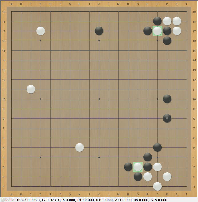 |
| Net correctly flags working ladders. No white stone is a ladder breaker. |
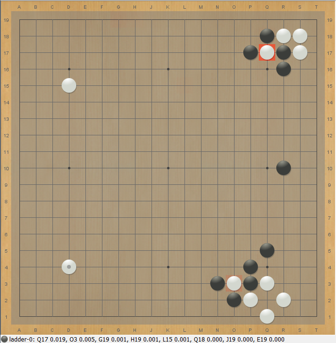 |
| Net correctly determines that ladders don't work. |
Update (Feb 2018):
Apparently, adding this block into the neural net does not cause it to be able to learn ladders in a supervised setting. From digging into the data a little, my suspicion is that in supervised settings, whether a ladder works or not is too strongly correlated with whether it gets formed in the first place, and similarly for escapes due to ladder breakers. So that unless it's plainly obvious whether the ladder works or not (the ladder-target experiments show this block makes it much easier, but it's still not trivial), the neural net fails to pick up on the signal. It's possible that in a reinforcement learning setting (e.g. Leela Zero), this would be different.
Strangely however, adding this block in did improve the loss, by about 0.015 nats at 5 million training steps persisting to still a bit more than 0.010 nats at 12 million training steps. I'm not sure exactly what the neural net is using this block for, but it's being used for something. Due to the bottlenecked nature of the block (I'm using only C = 6), it barely increases the number of parameters in the neural net, so this is a pretty surprising improvement in relative terms. So I kept this block in the net while moving on to later experiments, and I haven't gone back to testing further.
Using Ladders as an Extra Training Target (Feb 2018)
In another effort to make the neural net understand ladders, I added a second head to the neural net and forced the neural net to simultaneously predict the next move and to identify all groups that were in or could be put in inescapable atari.
Mostly, this didn't work so well. With the size of neural net I was testing (~4-5 blocks, 192 channels) I was unable to get the neural net to produce predictions of long-distance ladders anywhere near as well as it did when it had the ladder target alone, unless I was willing to downweight the policy target in the loss function enough that it would no longer produce as-good predictions of the next move. With just a small weighting on the ladder target, the neural net learned to produce highly correct predictions for a variety of local inescapable ataris, such as edge-related captures, throw-in tactics and snapbacks, mostly everything except long-distance ladders. Presumably due to the additional regularization, this improved the loss for the policy very slightly, bouncing around 0.003-0.008 nats around 5 to 10 million training steps.
But simply adding the ladder feature directly as an input to the neural net dominated this, improving the loss very slightly further. Also, with the feature directly provided as an input to the neural net, the neural net was finally able to tease out enough signal to mostly handle ladders well.
 |  |
| Extra ladder target training doesn't stop net from trying to run from working ladder (left), but directly providing it as an input feature works (right). | |
 |  |
| And on the move before, whether the ladder works clearly affects the policy. | |
However, even with such a blunt signal, it still doesn't always handle ladders correctly! In some test positions, sometimes it fails to capture stones in a working ladder, or fails to run from a failed ladder, or continues to run from a working ladder, etc. Presumably pro players would not get into such situations in the first place, so there is a lack of data on these situations.
This suggests that a lot of these difficulties are due to the supervised-learning setting, rather than merely difficulty of learning to solve ladders. I'm quite confident that in a reinforcement-learning setting more like the "Zero" training, with ladders actually provided directly as an input feature, the neural net would rapidly learn to not make such mistakes. It's also possible that in such settings, with a special ladder block the neural net would also not need ladders as an input feature and that the block would end up being used for ladder solving instead of whatever mysterious use it's currently being put to.
 |
| Even when told via input feature that this ladder works, the NN still wants to try to escape. |
Global Pooled Properties (Dec 2017)
Starting from a purely-convolutional policy net, I noticed a pretty significant change in move prediction accuracy despite only a small increase in the number of trainable parameters when I added the following structure to the policy head. The intent is to allow the neural net to compute some "global" properties of the board that may affect local play.
- Separately from the main convolutions that feed into the rest of the policy head, on the side compute C channels of 3x3 convolutions (shape 19x19xC).
- Max-pool, average-pool, and stdev-pool these C channels across the whole board (shape 1x1x(3C))
- Multiply by (3C)xN matrix where N is the number of channels for the convolutions for the rest of the policy head (shape 1x1xN).
- Broadcast the result up to 19x19xN and add it into the 19x19xN tensor resuting from the main convolutions for the policy head.
The idea is that the neural net can use these C global max-pooled or average-pooled channels to compute things like "is there currently a ko fight", and if so, upweight the subset of the N policy channels that correspond to playing ko threat moves, or compute "who has more territory", and upweight the subset of the N channels that match risky-move patterns or safe-move-patterns based on the result.
Experimentally, that's what it does! I tried C = 16, and when visualizing the activations 19x19xC in the neural net in various posititions just prior to the pooling, I found it had chosen the following 16 global features, which amazingly were mostly all humanly interpretable:
- Game phase detectors (when pooled, these are all very useful for distinguishing opening/midgame/endgame)
- 1 channel that activated when near a stone of either color.
- 1 that activated within a wide radius of any stone. (an is-it-the-super-early-opening detector)
- 1 that activated when not near a strong or settled group.
- 1 that activated near an unfinished territoral border, and negative in any settled territory by either side.
- Last-move (I still don't understand why these are important to compute to be pooled, but clearly the neural net thought they were.)
- 5 distinct channels that activated near the last move or the last-last move, all in hard-to-understand but clearly different ways
- Ko fight detector (presumably used to tell if it was time to play a ko threat anywhere else on the board)
- 1 channel that highlighted strongly on any ko fight that was worth anything.
- Urgency or weakness detectors (presumably used to measure the global temperature and help decide things like tenukis)
- 4 different channels that detected various aspects of "is moving in this region urgent", such as being positive near weak groups, or in contact fights, etc.
- Who is ahead? (presumably used to decide to play risky or safe)
- 1 channel that activated in regions that the player controlled
- 1 channel that activated in regions that the opponent controlled
So apparently global pooled properties help a lot. I bet this could also be done as a special residual block earlier in the neural net rather than putting it only in the policy head.
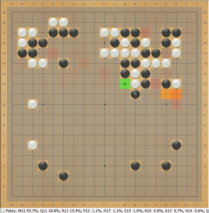
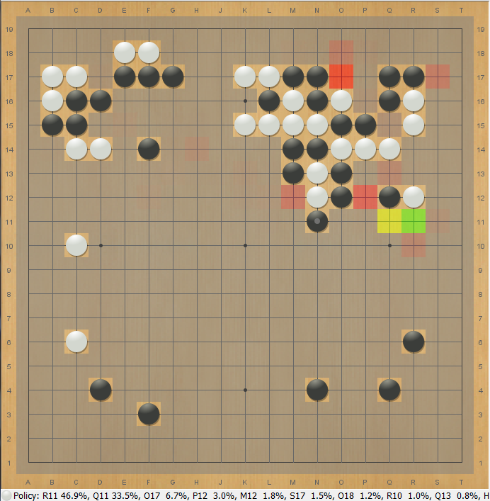
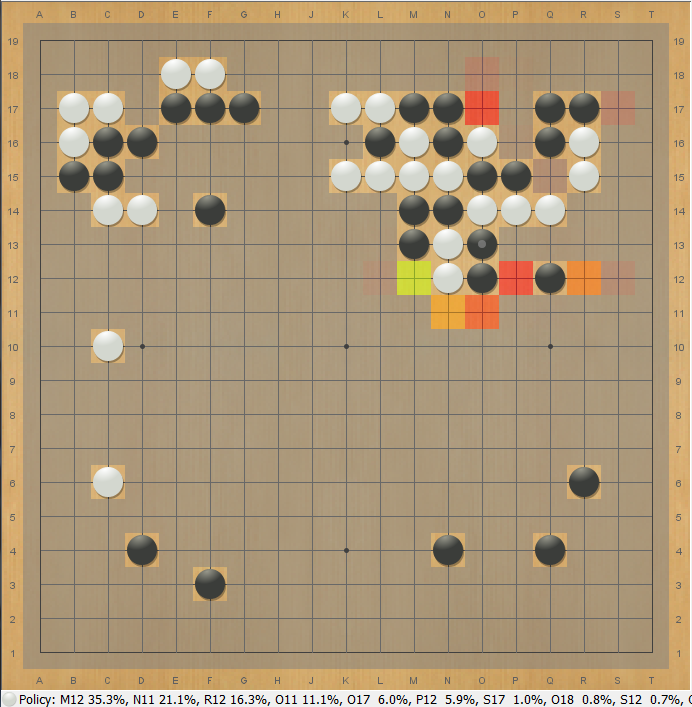
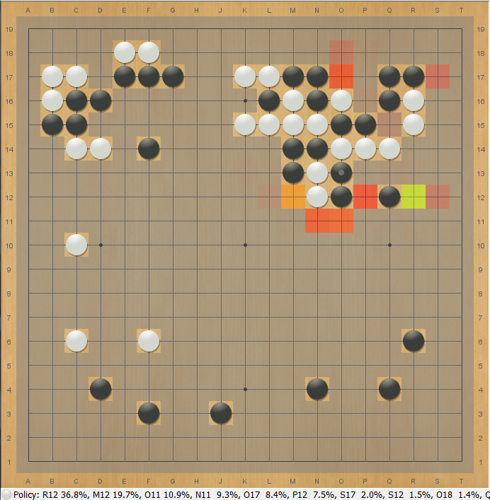
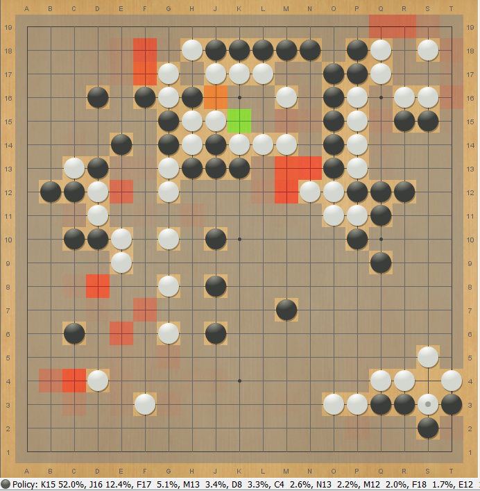
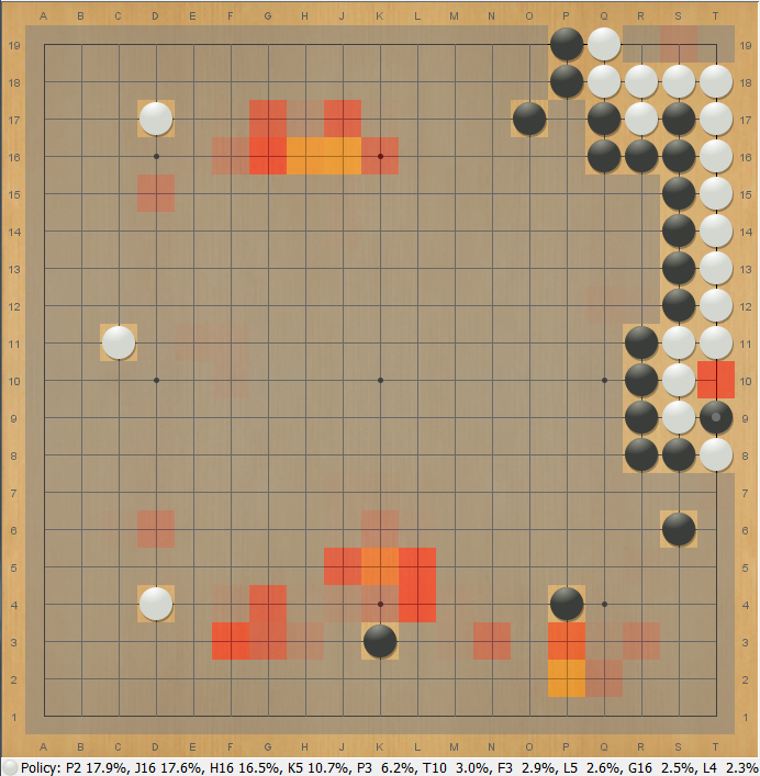
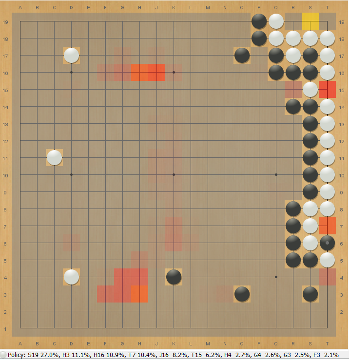
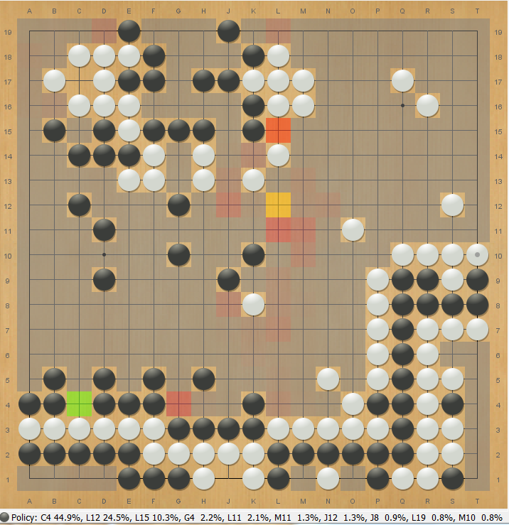
Here's a heatmap of the ko-fight detector channel, just prior to pooling. It activates bright green in this position after a ko was just taken. Everywhere else the heatmap is covered with checkerlike patterns, suggesting the kinds of shapes that the detector is sensitive to.
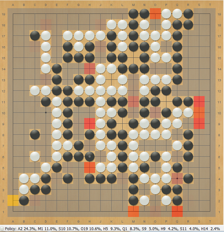
As a result of the pooling, the net predicts a distant ko threat:
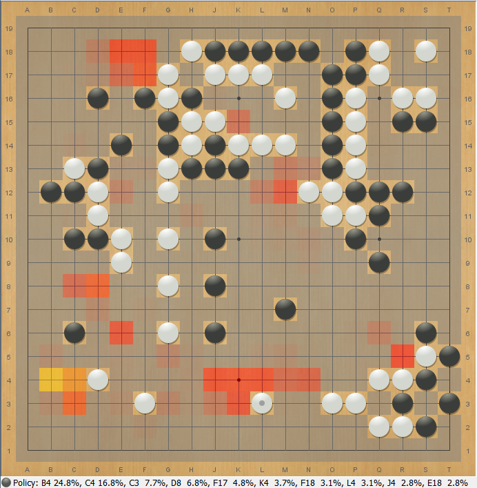
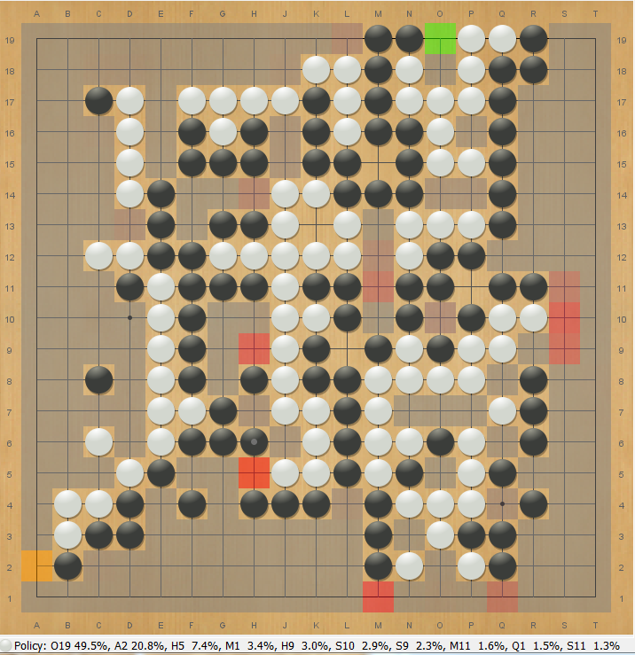
But when there is no ko, the net no longer wants to play ko threats:
Update (Feb 2018):
The original tests of global pooled properties was done when the neural net was an order of magnitude smaller than it is now (~250K params instead of ~3M params), so I did a quick test of removing this part of the policy head to sanity check if this was still useful. Removing it immediately worsened the loss by about 0.04 nats on the first several million training steps. Generally, differences early in training tend to diminish as the neural net converges further, but I would still guess at minimum 0.01 nats of harm at convergence, so this was a large enough drop that I didn't think it worth the GPU time to run it any longer.
So this is still adding plenty of value to the neural net. From a Go-playing perspective, it's also fairly obvious in practice that these channels are doing work. At least in ko fights, since the capture of an important ko plainly causes the neural net to suggest ko-threat moves all over the board that it would otherwise never suggest, including ones too far away to be easily reached by successive convolutions. I find it interesting that I haven't yet found any other published architectures include such a structure in the neural net.
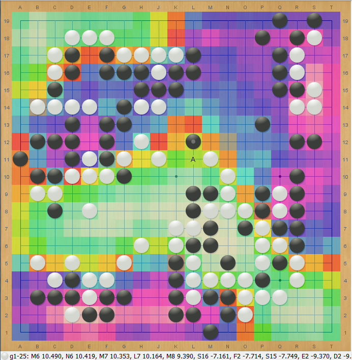
Just for fun, here's some more pictures of channels just prior to the pooling. These are from the latest nets that use parametric ReLU, so the channels have negative values now as well (indicated by blues, purples, and magentas).
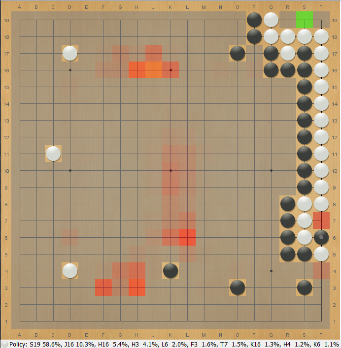
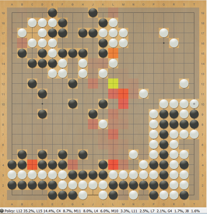
Despite only being trained to predict moves, this net has developed a rough territory detector! It also clearly understands the upper right white group is dead:
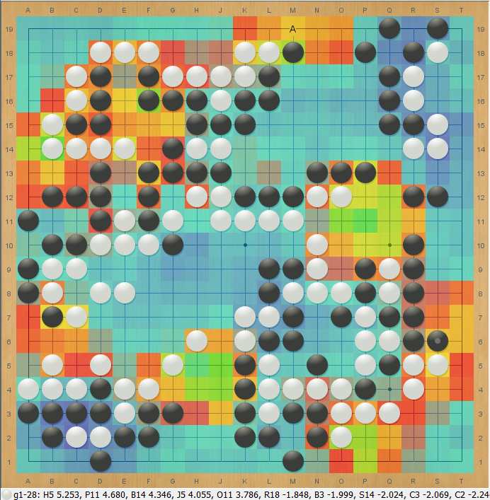
And this appears to be a detector for unfinished endgame borders:
Update (Mar 2018):
I experimented with these just a little more and found that the "stdev" part of the pooling doesn't seem to help. Only the average and max components are useful. Eliminating the stdev component of the pooling resulted in a few percent of performance improvement with no noticeable loss in prediction quality. If anything, it even improved slightly, although well within noise (on the order of 0.002 nats or less throughout training).
More importantly, it seems that global pooling is valuable as an addition to the main residual trunk, rather than just the policy head! I tested this out by replacing a few ordinary and dilated-convolution residual blocks with residual blocks structured similarly to the policy head - computing an extra convolution in parallel whose channels were then globally pooled, transformed, and then summed back with the first convolution's output, before being fed onward to the second convolution of the residual block as usual. For a 12-block net, augmenting two of the residual blocks this way resulted in a major 0.02 nats of improvement persisting at about 60 million training steps, while slightly decreasing the number of parameters and having no cost to performance.
One story for why global pooling might be effective in the main trunk is that there the computed features (such as global quantity of ko threats or game phase) can have a much more integrated effect on the neural net's predictions by adjusting its procesing of different shapes and tactics (for example, favoring or disfavoring moves that could lead to future ko fights). Whereas if the global pooling is deferred only until the policy head, the only thing the neural net can do with the information is the relatively cruder operation of precomputing a few fixed sets of moves it would want to play and simply upweighting or downweighting those sets of moves based on the global features.
As an aside, all the stats in the "current results" tables earlier were produced without this improvement, since I didn't think to try including global pooling in the trunk before all the other final experiments and test games were underway. While the apparent gain would likely continue to diminish with further training time, I expect some of the results would be yet slightly better if this were incorporated and everything re-run. (edit: as of Apr 2018, did add a row now in the stats table showing this).
Update (Apr 2018):
Just to get a proper comparison, I re-ran a proper training run with global pooling in the trunk rather than only the policy head on the GoGoD data set, along with some improvements to the learning rate schedule and updated the results table above. The difference is pretty large! Global pooling is by far the most successful architectural idea I"ve tried so far.
Update (Oct 2018):
Got around to testing the actual effect of global pooling on the strength of neural nets.
Elo Ratings by bot, 400 playouts
value33-140-400p-fpu20(gpool)  : 526.5  75cf ( 521.5, 531.5)  95cf ( 518.5, 534.5)  (4819.0 win, 4091.0 loss)
value45-140-400p-fpu20(nogpool): 449.7  75cf ( 436.7, 462.7)  95cf ( 425.7, 473.7)  (363.0 win, 564.0 loss)
value52-140-400p-fpu20(nogpool): 447.3  75cf ( 435.3, 459.3)  95cf ( 425.3, 468.3)  (450.0 win, 709.0 loss)

Elo Ratings by bot, 100 playouts
value33-140-100p-fpu20(gpool)  : 160.4  75cf ( 156.4, 164.4)  95cf ( 153.4, 167.4)  (7165.0 win, 6030.0 loss)
value52-140-100p-fpu20(nogpool): 107.2  75cf (  97.2, 117.2)  95cf (  89.2, 125.2)  (673.0 win, 913.0 loss)
value45-140-100p-fpu20(nogpool):  88.3  75cf (  77.3,  99.3)  95cf (  67.3, 108.3)  (512.0 win, 774.0 loss)
The "value45" and "value52" nets are two identical independent training runs, trained for 140M samples on LZ105-LZ142 and ELF games. Both are identical to "value33" except that the residual blocks that contain global pooling and the global pooling structure in the policy net have been removed, and in the case of the residual blocks, replaced with normal residual blocks.
As expected, global pooling appears to provide a modest but clear strength gain compared to not having it. Also as expected, separate performance testing indicated that there was very little performance cost to including the global pooling (the cost of pooling is minimal compared to convolution, and in this implementation the pooling channels actually replace some of the regular channels rather than being an addition to them). So this seems to be just a pure strength gain for the neural net.
Wide Low-Rank Residual Blocks (Feb 2018)
In one experiment, I found that adding a single residual block that performs a 1x9 and then a 9x1 convolution (as well as in parallel a 9x1 and then a 1x9 convolution, sharing weights) appears to decrease the loss slightly more than adding an additional ordinary block that does two 3x3 convolutions.
The idea is that such a block makes it easier for the neural net to propagate certain kinds of information faster across distance in the case where it doesn't need very detailed of nonlinear computations, much faster than 3x3 convolutions would allow. For example, one might imagine this being used to propagate information about large-scale influence from walls.
However, there's the drawback that either this causes an horizontal-vertical asymmetry if you don't do the convolutions in both orders of orientations, or else this block costs twice in performance as much as an ordinary residual block. I suspect it's possible to get a version that is more purely benefiting, but I haven't tried a lot of permutations on this idea yet, so this is still an area to be explored.
Parametric ReLUs (Feb 2018)
I found a moderate improvement when switching to using parametric ReLUs (https://arxiv.org/pdf/1502.01852.pdf) instead of ordinary ReLUs. I also I found a very weird result about what parameters it wants to choose for them. I haven't heard of anyone else using parametric ReLUs for Go, so I'm curious if this result replicates in anyone else's neural nets.
 |
| Left: ordinary ReLU. Right: parametric ReLU, where "a" is a trainable parameter. Image from https://arxiv.org/pdf/1502.01852.pdf |
For a negligible increase in the number of parameters of the neural net, using parametric ReLUs improved the loss by about 0.025 nats over the first 5 million training steps, a fairly significant improvement given the simplicity of the change. This decayed to little to closer to 0.010 to 0.015 nats by 15 million training steps, but was still persistently and clearly better, well above the noise in the loss between successive runs.
As far as I can tell, this was not simply due to something like having a problem of dead ReLUs beforehand, or some other simple issue. Ever since batch normalization was added, much earlier, all stats about the gradients and values in the inner layers have indicated that very few of the ReLUs die during training. Rather, I think this change is some sort of genuine increase in the fitting ability of the neural net.
The idea that this is doing something useful for the net is supported by a strange observation: for the vast majority of the ReLUs, it seems like the neural net wants to choose a negative value for a! That means that the resulting activation function is non-monotone. In one of the most recent nets, depending on the layer, the mean value of a for all the ReLUs in a layer varies from around -0.15 to around -0.40, with standard deviation on the order of 0.10 to 0.15.
With one exception: the ReLUs involved in the global pooled properties layer persistently choose positive a, with a mean of positive 0.30. If any layer were to be different, I'd expect it to be this one, since these values are used in a very different way than any other layer, being globally pooled before being globally rebroadcast. Still, it's interesting that there's such a difference.
For the vast majority of the ReLUs though, as far as I can tell, the neural net actually does "want" the activation to be non-monotone. In a short test run where a was initialized to a positive value of 0.25 rather than 0, the neural net over the course of the first few million training steps forced all the as to be negative mean again, except for the ones in the global pooled properties layer. In the meantime, it also had a larger training loss indicating that it was not fitting as well due to the positive as.
I'd be very curious to hear whether this reproduces for anyone else. For now, I've been keeping the parametric ReLUs, since they do seem to be an improvement, although I'm quite mystified about why non-monotone functions are good here.
Update - Parametric ReLU instability in Value Head (Jul 2018):
(this section accidentally omitted from an earlier update, only actually added later in September).
More recently once I added a value head to my neural net and began training on Leela Zero data, I found that parametric ReLUs seem to contribute to instability in the training of the value head. Here is a graph of the validation loss of the value head of four 12-block neural nets trained on LZ128-LZ142 + ELF over the first 100 million training data samples. Two of them used PReLU, and two of them did not. (note: among one of the two that did, there is a slight head architecture difference that I was also testing at the time, but it doesn't appear to have much effect, otherwise all architectures and hyperparameters are the same except for use of PReLU vs ReLU).
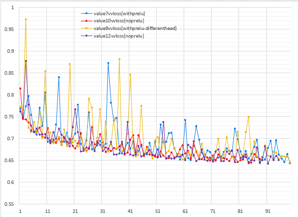 |
| X-Axis: Number of millions of training samples. Y-Axis: Validation loss |
Looking at the graph, the two training runs that used PReLU have the validation loss of the value head jump around quite a lot more than the two that used plain ReLU. I have no idea why this is the case. Additionally, the gain from PReLU seems to be much smaller and/or hard to distinguish from noise compared to when I first tested it, possibly due to the fact that these neural nets are a much larger 12 blocks than when I initially tested with 5 blocks. So for now, I'm gone back to not using them.
Chain Pooling (Feb 2018)
Using the following functions:
- https://www.tensorflow.org/api_docs/python/tf/unsorted_segment_max
- https://www.tensorflow.org/api_docs/python/tf/gather
...it's possible to implement a layer that performs max-pooling across connected chains of stones (rather than pooling across 2x2 squares as you normally see in the image literature).
I tried adding a residual block that applied this layer, and got mixed results. On the one hand, when trying the resulting neural net in test cases, it improves all the situations you would expect it to improve.
For example, an ordinary neural net has no problem with making two eyes in this position when its lower eye is falsified:
But, when you make it too far away, the neural net doesn't have enough convolutional layers to propagate the information, so it no longer suggests S19 to live:
Adding a residual block with a chain pooling layer improves this, the neural net now suggests to live even when the move is arbitrarily far away, as long as the group is solidly connected:
And even does so partially when there's a gap in the chain, since the chain pooling is still able to propagate the information a good distance.

I've also observed improvements in a variety of other cases, particularly in large capturing races or in endgame situations where a filled dame on a large chain requires a far-away defense. In all these cases, chain-pooling helped the neural net find the correct response.
However, when I added a single chain pooling residual block with a small number of channels (32 channels), the loss actually got worse by a significant 0.010 nats even all the way out to 64 million training steps. And in self-play, the overall playing strength was not obviously better, winning 292 games out of 600 against the old neural net. I don't know exactly what's going on that makes the neural net solve races and liberty situations better in test positions but not be noticeably better, perhaps either these positions are just rare and not so important, or perhaps the chain pooling is causing the rest of the neural net to not fit as well for some reason.
When I added two chain pooling blocks each with 64 channels, this time the loss did get better, but only by about 0.005 nats at 10 million training steps, which would presumably decay a little further as the neural net converged, which was still underwhelming.
One additional problem is that the chain pooling is fairly computationally expensive compared to plain convolutional layers. I haven't done detailed measurements, but it's probably at least several times more expensive, so even with an improvement it's not obvious that this is worth it over simply adding more ordinary residual blocks.
So all the results in test positions looked promising, but the actual stats on performance and improvement in the loss were a bit disappointing. I'll probably revisit variations on this idea later, particularly if I can find a cheaper way to compute something like this in Tensorflow.
Dilated Convolutions (Mar 2018)
It turns out that there's a far better approach than chain pooling to help the neural net to propogate information across larger distances, which is the technique of dilated convolutions. As described in https://arxiv.org/pdf/1511.07122.pdf, dilated convolutions are like regular convolutions except that the patch of sampled values, in our case 3x3, is not a contiguous 3x3 square, but rather is composed of 9 values sampled at a wider spacing, according to a dilation factor > 1. The idea, obviously, is that the neural net can see farther with the same number of layers at the cost of some local discrimination ability.
I experimented with this by taking the then-latest neural net architecture and for each residual block after the first, altering 64 of the 192 channels of the first convolution in the block to be computed via dilated convolutions with dilation factors of 2 or 3 instead of regular convolutions (dilation factor = 1). The results were very cool; the neural net improved on all the same kinds of situations that chain pooling helped with, enabling the neural net to understand much longer-distance relationships and perceive the status of larger groups correctly:
 |  |
| Left: 5-block net fails to reply to throw-in by making eyes in the upper right.
Right: 5-block with dilated convolutions succeeds. | |
 |  |
| Left: 5-block net fails to respond to eye-poke by making eye up top.
Right: 5-block with dilated convolutions succeeds. | |
 |  |
| Left: 5-block net fails to reply to distant liberty fill in a capturing race.
Right: 5-block with dilated convolutions succeeds. | |
Presumably, the neural net learned in its first few layers to compute features that indicate when there is connectivity with stones at distance 2 or 3, which then are used by the dilated convolutions to propagate information about liberties and eyes 2 or 3 spaces per convolution, rather than only 1 space at a time.
Like chain pooling, holding the number of parameters constant I did not find it to noticeably improve the cross-entropy loss. However when replacing 64/192 of the channels in this way, the loss also did not get worse either, unlike how it would definitely get worse if one were to simply delete those channels. Combined with the above pictures, it suggests the neural net is putting the dilations to good use to learn longer-distance relationships at the cost of being a little worse at some local shapes or tactics. And unlike chain pooling, dilated convolutions appear to be quite cheap, barely at all increasing the computational cost of the neural net.
So unlike chain pooling, this technique still seems quite promising and worth experimenting with further. For example, I haven't done any testing on whether this improves the overall quality of the neural net for use within MCTS. Many of the deep-learning generation of Go bots, before they reach AlphaGo-levels of dominance, appear to have their biggest weaknesses in the perception of large chains or large dragons and understanding their liberty or their life and death status. Recently also the literature appears to be filled with results like https://openreview.net/forum?id=HkpYwMZRb that suggest that the "effective depth" of neural nets does not scale as fast as their physical depth. This also might explain why it's slow for neural nets like those of AlphaGo Zero and Leela Zero to learn long-distance effects even when they have more than enough physical depth to eventually do so. These seem like precisely the kinds of problems that dilated convolutions could help with, and it's plausible that on the margin the tradeoff of making local shape understanding a bit worse in exchange would be good (as hopefully the search could correct for that).
Dilated Convolutions - Effect on Playing Strength (Oct 2018)
Tried testing the actual effect of dilated convolution on playing strength.
Elo Ratings by bot, 400 playouts
value33-140-400p-fpu20(dilated)  : 526.5  75cf ( 521.5, 531.5)  95cf ( 518.5, 534.5)  (4819.0 win, 4091.0 loss)
value44-140-400p-fpu20(nodilated): 505.5  75cf ( 493.5, 517.5)  95cf ( 484.5, 526.5)  (537.0 win, 606.0 loss)
value43-140-400p-fpu20(nodilated): 502.0  75cf ( 492.0, 512.0)  95cf ( 484.0, 520.0)  (714.0 win, 822.0 loss)

Elo Ratings by bot, 100 playouts
value33-140-100p-fpu20(dilated)  : 160.4  75cf ( 156.4, 164.4)  95cf ( 153.4, 167.4)  (7165.0 win, 6030.0 loss)
value43-140-100p-fpu20(nodilated): 141.4  75cf ( 131.4, 151.4)  95cf ( 123.4, 159.4)  (792.0 win, 883.0 loss)
value44-140-100p-fpu20(nodilated): 136.0  75cf ( 126.0, 146.0)  95cf ( 118.0, 154.0)  (726.0 win, 835.0 loss)
The "value43" and "value44" nets are two identical independent training runs, trained for 140M samples on LZ105-LZ142 and ELF games. Both are identical to "value33" except that all convolutions have dilation factor 1, whereas "value33" has 64/192 of the channels within the first convolution of each residual block have dilation factor 2. It appears that there maybe a very slight strength gain from having dilated convolutions, holding playouts constant, although the gain is small enough that if real, it is only on a similar level to the random variation between different training runs. And unfortunately, some informal performance testing suggests that dilated convolutions appear to have a noticeable performance cost relative to dilated convolutions in cuDNN, and also do not benefit from FP16 tensor cores for GPUs that have them. This makes them problematic.
Additionally, all three neural nets have already enough layers to see well across the board regardless (14 blocks), so a-priori one might expect the gains from dilated convolutions to be limited. Given this fact and the performance costs, they seem unpromising at this point, although they would likely still be worth testing further in a context where dilated convolutions were cheaper (maybe CPU implementations, or some other GPU implementations?) and for smaller neural nets for lighter-weight devices that cannot afford a number of blocks so as to easily see far across the board.
Redundant Parameters and Learning Rates (Feb 2018)
There is a class of kinds of twiddles you can do to the architecture of a neural net that are completely "redundant" and leave the neural net's representation ability exactly unchanged. In many contexts I've seen people completely dismiss these sorts of twiddles, but confusingly, I've noticed that they actually can have effects on the learning. And sometimes in published papers, I've noticed the authors use such architectures without any mention of the redundancy, leaving me to wonder how widespread the knowledge about these sorts of things is.
Redundant Convolution Weights
For example, in one paper on ResNets in Go, (http://www.lamsade.dauphine.fr/~cazenave/papers/resnet.pdf), for the initial convolution that begins the residual trunk, the author chose to use the sum of a 5x5 convolution and a 1x1 convolution. One might intuit this change to be potentially good, since the first layer will probably often not be computing overly sophisticated 5x5 patterns, and a significant amount of its job will be computing various important logical combinations of the input features to pass through (e.g. "stone has 1 liberty AND is next to the opponent's previous move") that will frequently involve the center weight, so the center weights will be important more often than the edge weights.
However, adding a 1x1 convolution to the existing 5x5 is completely redundant, because that's equivalent to doing only a 5x5 convolution with a different central weight.
Adding the results of two separate convolutions with these kernels:
a   b   c   d   e
f   g   h   i   j
k   l   m   n   o                z
p   q   r   s   t
u   v   w   x   y

Is the same as doing a single convolution with this kernel:
a   b   c   d   e
f   g   h   i   j
k   l (m+z) n   o
p   q   r   s   t
u   v   w   x   y
Nonetheless, it has an effect on the learning. With standard weight initialization, this causes the center weight in the equivalent single 5x5 kernel to be initialized much larger on average. For example I think Xavier initialization will initialize z to be sqrt(25) = 5 times larger on average than m. Moreover, during training, the learning rate of the center weight in the kernel is effectively doubled, because now m and z will both experience the gradient, and when they each take a step, their sum will take twice as large of a step.
So in my own neural nets I tried adding an additional parameter in the center of the existing 5x5 convolution, and in fact, it was an improvement! Only about 0.01 nats in early training, decaying to a slight improvement of less than 0.005 nats by 25 million training steps. But still an improvement to the overall speed of learning.
(The current neural nets in this sandbox use a 5x5 convolution rather than a 3x3 to begin the ResNet trunk since the small number of channels of the input layer makes it uniquely cheap to do a larger convolution here, unlike the rest of the neural net with 192 channels. It probably helps slightly in kicking things off, such as being able to detect the edge from 2 spaces away instead of only 1 space away by the start of the first residual block.)
I haven't gotten to it yet, but in the future I want to test more changes of this flavor. For example, given that it was a good idea to increase the weight initialization and learning rate on the center weight for the initial 5x5 convolution, could it be a good idea to do the same for all the 3x3 convolutions everywhere else in the neural net?
Update (Mar 2018):
Apparently, it is a good idea! Emphasizing the center weight initialization by 30% and increasing the learning rate by a factor of 1.5 on the center weight for the other convolutions in the neural net improved the rate of learning in one test giving about an 0.01 nat improvement at around 50 million training samples.
Also, to confirm the intuition behind this idea, I looked in a neural net trained without any special center emphasis at the average norm of the learned convolution weights by position within the convolution kernel. Here is a screenshot of the average norm of the weights for the first 4 residual blocks of a particular such net, displayed with coloring in a spreadsheet:
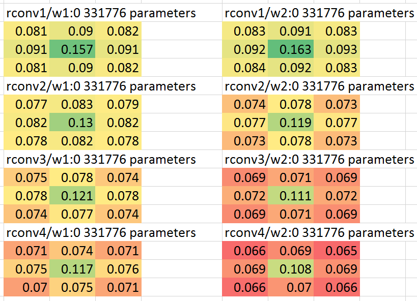
So on its own, the neural net chooses on average to put more weight in the center than on the edges or corners of the 3x3 convolutions. So it's not surprising that allowing the neural net to adjust the center weight relatively more rapidly than the other weights is an improvement for learning speed, even if, as I suspect, in ultimate convergence it might not matter.
Batch Norm Gammas
Another redundancy I've been experimenting with is the fact that due to historical accident, the current neural nets in this sandbox use scale=True in batch norm layers, even though the resulting gamma scale parameters are completely redundant with the convolution weights afterwards. This is because ReLUs (and parametric ReLUs) are scale-preserving, so a neural net having a batch norm layer with a given gamma is equivalent to one without gamma but where the next layer's convolution weights for that incoming channel are gamma-times-larger.
Yet, despite the redundancy, the presence of those redundant parameters does influence the learning. In some quick tests I was not able to get rid of them. Although I didn't try so extensively, in a handful of tries I was unable to find a combination of setting scale=False and increasing the learning rate to compensate that did not slow down the total efficiency of learning. So the latest neural nets for now continue to use scale=True.
Update (Apr 2018):
Since it's been a long time, I re-tested this again and was able to eliminate these. I'm not exactly sure what the difference was this time versus the previous attempt, or maybe the previous attempt found a difference only due to confounding noise between different initializations. It might be worth exploring this kind of detail further though. What, theoretically, should one expect the effect of having this particular kind of redundancy to have on the learning?
Some Thoughts About History as an Input (Mar 2018)
Most or all of the open-source projects I've seen that aim to reproduce Alpha-Zero-like training seem to have the issue that the resulting neural net requires the history of the last several moves as input to the neural net. This somewhat limits the use of these bots for analysis, whether for whole-board tsumego or for asking of "what if" questions such as analyzing with/without an extra local stone, or for seeing in kyu-level games what the policy net would suggest without the presumption that the opponent's move was a good move (as would be in nearly all later games composing the training data).
I just wanted to record here that there is a very simple solution which I've used successfully so far to enable the neural net to also play well without history and that hardly costs anything. You simply take a small random percentage of positions in training, say 5%-10%, and don't provide the history information on those positions.
- If you're using binary indicators of the locations of past moves and captures, this corresponds to zeroing out those planes.
- If you're using the AlphaGoZero representation where you give whole past board states rather than giving binary indicators of recent moves, it's probably better to make the past board states to be unchanged copies of the current board state rather than zeroing them, since having them be identical is the closest way to say that no local moves happened there. (As opposed to zeroing them, which would be like telling the net that every stone was suddenly and recently placed).
Now, since you have training examples without history, the neural net adapts to produce reasonable predictions without history. But since nearly all the training examples still do have history, the neural net still mostly optimizes for having history and should lose little if any strength there.
Also, I wonder if there might be room for further experimentation along these lines. In general, normal methods of training the policy part of a net will cause it to learn that moves provided in its history represent strong play, because all examples in its training data have that property. However in many branches of an MCTS search, or when used as an analysis tool, this is definitely not the case. This may cause the policy to be too obedient in response to bad moves ("a strong opponent wouldn't have played here unless it was sente") and make the search less effective at refuting them (by tenukiing).
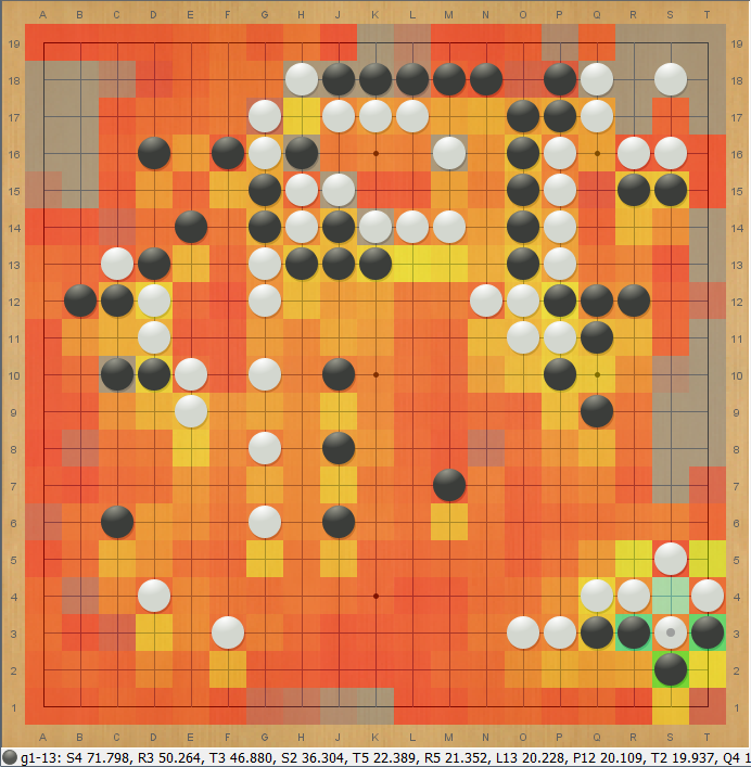
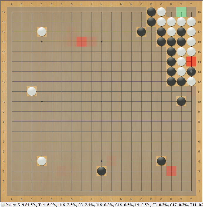
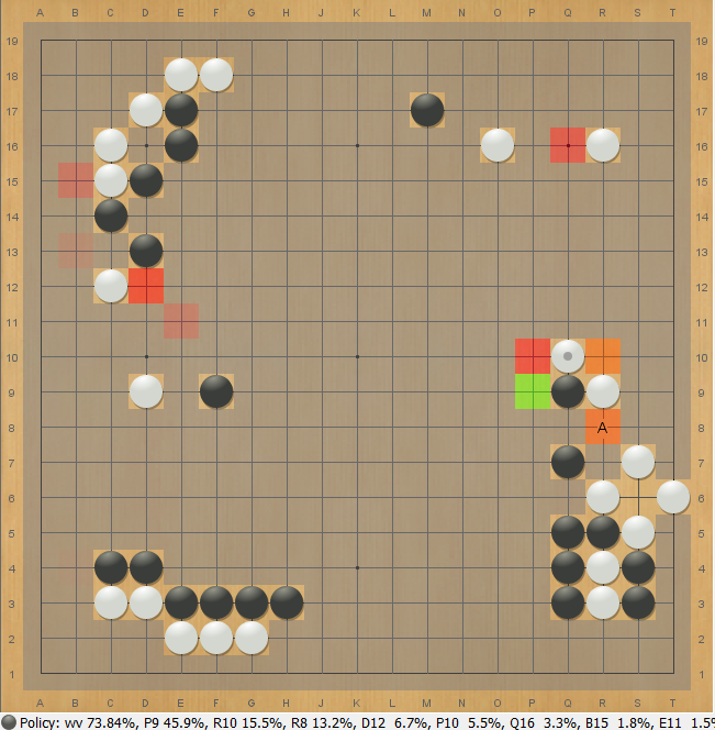
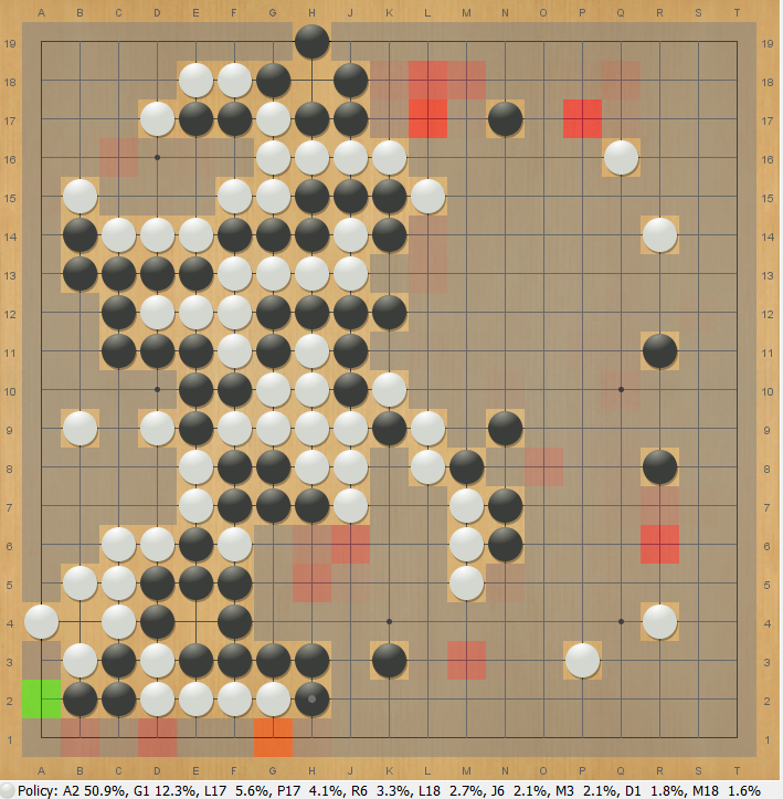 | 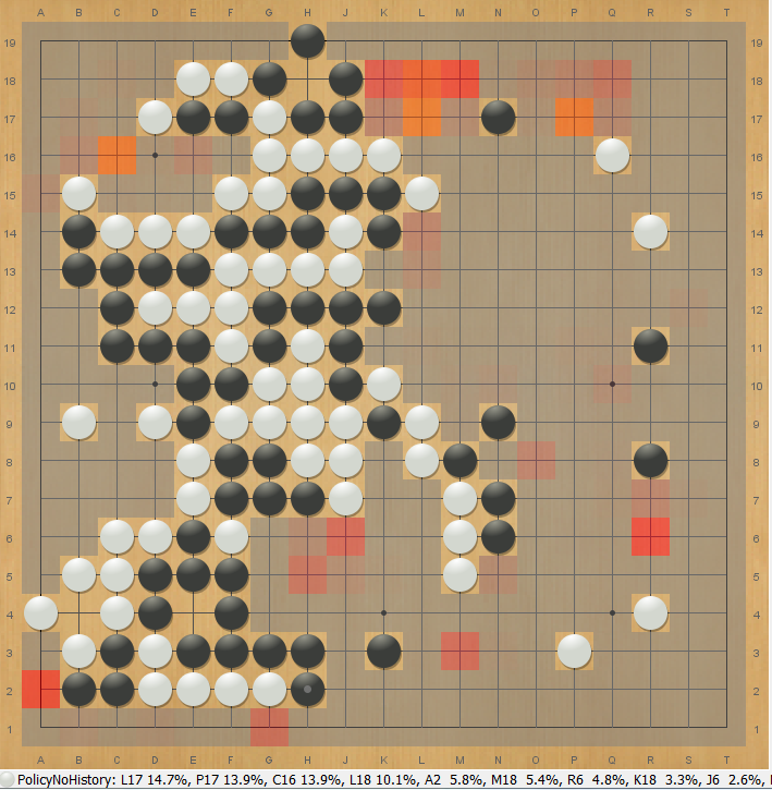 |
| Left: With history, net wants to unnecessarily respond to black's slow gote move in the lower left.
Right: With move history planes zeroed out, net suggests moves in the more urgent areas at the top. | |
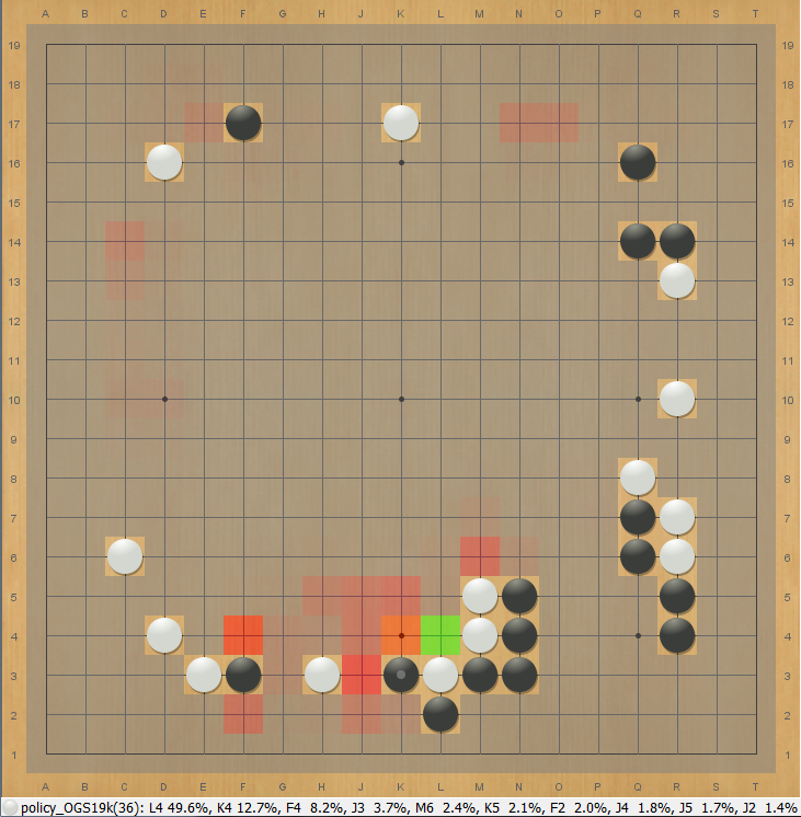
Ranks as an Input (June 2018):
I added the rank of the player of the moves being predicted as an input to the neural net. A total of 64 different (rank * online server) combinations are provided to the neural net as a one-hot-encoded vector, which passes through an 8-dimensional embedding layer before being combined with the rest of the board features. As a result, the neural net can learn to predict how players of different strengths play differently!
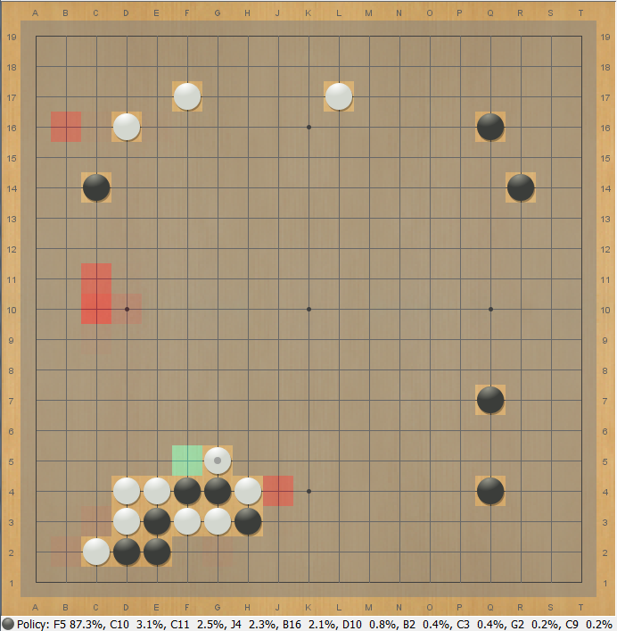
As an example, in this position, it thinks that a typical 19 kyu (OGS) player would most likely connect against black's atari:
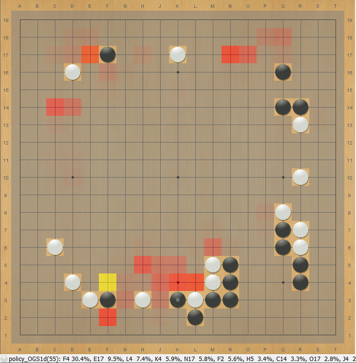
But a 1 dan player would more likely prefer to sacrifice those stones and complete the lower left shape:
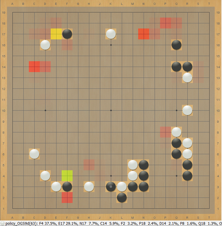
And the net thinks a 9 dan player would be likely to do the same, but might also likely tenuki to the upper left, which is also reasonably urgent:
Using this neural net and a bunch of heuristic filtering criteria, I found a way to generate surprisingly reasonable whole-board open-space fighting and shape problems, which I posted here as a training tool for Go players: neuralnetgoproblems.com.
MCTS (Aug 2018):
After a dense couple months of work, I finished an efficient multithreaded MCTS implementation! The implementation supports batching of calls to the GPU both within a single search and across searches. The latter is useful for accelerating data gathering for testing, for example it can run N games in parallel, each one performing a single-threaded search, but where neural net evaluations across all the searches for all the games are batched, noticeably increasing throughput on high-end GPUs.
As a starting point, I began with similar parameters and logic to Leela Zero for handling first play urgency and minor other search details, but have further experimented since then. So far, I've been testing by running many different round-robin tournaments involving a wide range of versions of bots with different parameter settings, different neural nets, and different numbers of playouts (most of which are not displayed here), and feeding all the results through BayesElo, or rather a customized implementation of it.
The following test shows that the strength of play scales massively and rapidly with the number of root playouts, suggesting that the search is working well and at least does not contain any massive bugs:
Elo ratings by bot
value33-140-1200p :  843.8  75cf ( 830.8, 856.8)  95cf ( 820.8, 866.8)  (607.0 win, 477.0 loss)
value33-140-400p  :  417.7  75cf ( 409.7, 425.7)  95cf ( 402.7, 432.7)  (1397.0 win, 1892.0 loss)
value33-140-100p  :   26.0  75cf (  20.0,  32.0)  95cf (  16.0,  37.0)  (3984.0 win, 2206.0 loss)
value28-140-100p  :   22.3  75cf (  15.3,  30.3)  95cf (   9.3,  35.3)  (1817.0 win, 1439.0 loss)
value28-140-50p   : -186.3  75cf (-212.3,-160.3)  95cf (-235.3,-138.3)  (219.0 win, 151.0 loss)
value28-140-25p   : -337.2  75cf (-359.2,-316.2)  95cf (-378.2,-298.2)  (201.0 win, 446.0 loss)
value28-140-12p   : -525.9  75cf (-552.9,-499.9)  95cf (-576.9,-477.9)  (123.0 win, 528.0 loss)
value28-140-6p    : -745.3  75cf (-780.3,-713.3)  95cf (-810.3,-684.3)  ( 57.0 win, 588.0 loss)
value28-140-3p    : -893.6  75cf (-937.6,-855.6)  95cf (-976.6,-821.6)  ( 25.0 win, 623.0 loss)
Displayed above are the stats for the bots in those tournaments where primarily I was testing the effect of varying the number of playouts (with tree reuse, the actual size of the search tree will often be a little larger). "value28-140" and "value33-140" are neural nets trained on Leela Zero games LZ105-LZ142 and ELF games as of about June 27 for 141 million training samples, differing only in some insignificant simplifications to the head architecture. They have both converged well and appear to be well within statistical noise of each other in strength. You can see in the table above the maximum likelihood Elo ratings of these bots ranging from 3 playouts to 1200 playouts given the data assuming the standard Elo rating model where the probability of a win given a certain rating difference follows a logistic curve scaled so that 400 points difference implies to a 10:1 odds.
Also displayed are the symmetric 75% and 95% confidence intervals for each given bot assuming all other bots' Elo ratings are taken as given (so it does not account for the joint uncertainty or covariance between the various bot ratings, but is still a good indicator of the error bounds on these ratings). Several of the bots have many more games than the others, this is because those bots also participated in many other round robin tournaments against other bots not shown.
One might worry about the accuracy of the Elo model, or about nontransitivity effects distorting the stats when pooling all test games together into a shared BayesElo, In practice I haven't run into any noticeable problems doing this. So far, the only major caveat is that probably all these ratings differences are very inflated as is typical of self-play relative to what they would be against humans or against other bots trained on data that is sufficiently different.
Cross Entropy vs L2 Value Head Loss (Aug 2018):
After finishing the implementation of MCTS, like other some people have tried, I tried testing to see what effect if any that cross entropy versus L2 loss has for the value head of the neural net. In practice, I found I needed to multiply the cross entropy loss by 1.4 (treating the problem as a binary classification) to get it to have a roughly similar typical gradient magnitude as the L2 loss (treating the problem as a regression to a target of +1 or -1).
I trained neural nets to use a weighted average of the L2 loss and the 1.4x rescaled cross entropy loss, with 0%, 25%, 50%, and 100% weight on the cross entropy loss for the value head (and correspondingly 100%, 75%, 50%, and 0% on L2 loss). Here are the results:
Elo ratings by bot
value33-140-100p(ce50'')   :  26.0  75cf (  20.0,  32.0)  95cf (  16.0,  37.0)  (3984.0 win, 2206.0 loss)
value35-140-100p(ce100'')  :  23.0  75cf (  15.0,  31.0)  95cf (   9.0,  37.0)  (1445.0 win, 1231.0 loss)
value28-140-100p(ce50')    :  22.3  75cf (  15.3,  30.3)  95cf (   9.3,  35.3)  (1817.0 win, 1439.0 loss)
value21-140-100p(ce50)     :  17.8  75cf (   9.8,  25.8)  95cf (   3.8,  31.8)  (1700.0 win, 1371.0 loss)
value31-140-100p(ce0'')    :   7.6  75cf (  -0.4,  15.6)  95cf (  -7.4,  22.6)  (1295.0 win, 1202.0 loss)
value18-140-100p(ce0)      :  -0.0  75cf (  -9.0,   9.0)  95cf ( -16.0,  16.0)  (1203.0 win, 1352.0 loss)
value30-140-100p(ce25')    :  -1.5  75cf (  -9.5,   6.5)  95cf ( -15.5,  12.5)  (1570.0 win, 1357.0 loss)
value24-140-100p(ce0')     :  -4.8  75cf ( -13.8,   4.2)  95cf ( -20.8,  11.2)  (1261.0 win, 1087.0 loss)
value20-140-100p(ce0)      :  -8.5  75cf ( -17.5,   0.5)  95cf ( -25.5,   8.5)  (1128.0 win, 971.0 loss)
value32-140-100p(ce25'')   :  -8.7  75cf ( -17.7,   0.3)  95cf ( -24.7,   7.3)  (1019.0 win, 1046.0 loss)
value29-140-100p(ce50)     : -16.3  75cf ( -25.3,  -7.3)  95cf ( -33.3,   0.7)  (1071.0 win, 961.0 loss)
value26-140-100p(ce25')    : -46.2  75cf ( -55.2, -37.2)  95cf ( -62.2, -30.2)  (1106.0 win, 1196.0 loss)
value19-140-100p(ce100)    : -47.8  75cf ( -56.8, -38.8)  95cf ( -64.8, -30.8)  (1016.0 win, 1090.0 loss)
value34-140-100p(ce100'')  : -51.1  75cf ( -62.1, -40.1)  95cf ( -71.1, -31.1)  (559.0 win, 728.0 loss)
And a test at 400 playouts for a subset of those nets:
Elo ratings by bot
value33-140-400p(ce50'')   : 417.7  75cf ( 409.7, 425.7)  95cf ( 402.7, 432.7)  (1397.0 win, 1892.0 loss)
value31-140-400p(ce0'')    : 381.2  75cf ( 366.2, 396.2)  95cf ( 353.2, 409.2)  (413.0 win, 308.0 loss)
value32-140-400p(ce25'')   : 355.3  75cf ( 340.3, 370.3)  95cf ( 327.3, 383.3)  (385.0 win, 337.0 loss)
value34-140-400p(ce100'')  : 271.8  75cf ( 255.8, 287.8)  95cf ( 242.8, 299.8)  (298.0 win, 425.0 loss)
The various ' and '' marks indicate slight tweaks to the head architecture of the neural net that I made concurrently in order to make the CUDA code implementing that architecture cleaner and more maintainable, they do not appear to affect the strength of the net in a statistically noticeable way.
The results are pretty mixed, but I would say there are a few conclusions that one can tentatively draw:
- Neural nets trained under identical conditions can vary noticeably in overall strength.
- For example, value29-140-100p and value21-140-100p were trained under exactly identical conditions for for the same number of steps, differing only in the random initialization of their weights and the randomized order of the data batches during training. They ended up about 34 Elo apart, about 4 times the standard deviation of the uncertainty given the number of testing games played.
- The biggest difference between two identically-trained nets was value34-140-100p and value35-140-100p, ending up 74 Elo apart.
- This means that any strength test regarding architectural differences in a neural net needs to be repeated with many independently-trained versions of that neural net, it is only weak evidence to run such a test once.
- Putting some weight on cross entropy loss does not appear to harm the neural net on average. It is perhaps the case (not very certain) that putting a high weight on the cross entropy increases the variability of the neural net's final performance, as the higher cross-entropy-weighted nets seemed to finish near the top and near the bottom of the ratings more often.
- More playouts appears to exaggerate strength differences between neural nets caused by cross entropy versus L2 training.
It's interesting that there was no overall statistically clear effect on average neural net strength between cross entropy and L2 value head training given that direct inspection of the neural nets' behavior on actual positions suggests that the two losses do cause the neural net behave in different ways. Theoretically, one would expect cross entropy loss to cause the neural net to "care" more about accurate prediction for tail winning probabilities, and in fact this manifests in quite a significant difference in average "confidence" of the neural net on about 10000 test positions from the validation set:
Neural Net              sqrt(E(value prediction logits^2))
value31-140(ce0'')       1.09945
value32-140(ce25'')      2.04472
value33-140(ce50'')      2.22901
value35-140(ce100'')     2.28122
And indeed by manual inspection the cross-entropy neural nets seem to be much more willing to give more "confident" predictions:
 | 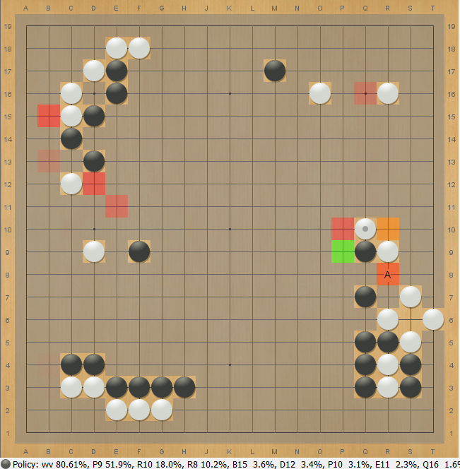 | 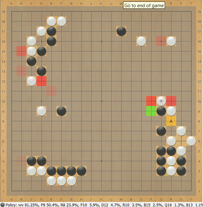 |
| White winrate rises from 74% to 81% to 91% between nets trained with 0%, 50%, 100% cross entropy. | ||
First Play Urgency (Aug 2018):
At the moment, the search uses much the same square-root-policy-net-based first-play urgency reduction that Leela Zero uses:
V(unvisited child) = ValueNet(parent) - k * sqrt( sum_{c: visited children} PolicyNet(c) )
I experimented briefly with using the average parent evaluation so far in the search as the base:
V(unvisited child) = MCTSValue(parent) - k * sqrt( sum_{c: visited children} PolicyNet(c) )
This seems more natural to me, but if anything, it seems to cause a very slight strength loss, at least at the numbers of visits tested:
Elo ratings by bot
value33-140-400p        : 417.7  75cf ( 409.7, 425.7)  95cf ( 402.7, 432.7)  (1397.0 win, 1892.0 loss)
value33-140-400p-pavg   : 403.9  75cf ( 395.9, 412.9)  95cf ( 388.9, 418.9)  (1280.0 win, 1143.0 loss)
value33-140-100p        :  26.0  75cf (  20.0,  32.0)  95cf (  16.0,  37.0)  (3984.0 win, 2206.0 loss)
value33-140-100p-pavg   :   9.8  75cf (   3.8,  15.8)  95cf (  -0.2,  19.8)  (3003.0 win, 3250.0 loss)
value31-140-100p        :   7.6  75cf (  -0.4,  15.6)  95cf (  -7.4,  22.6)  (1295.0 win, 1202.0 loss)
value31-140-100p-pavg   :  -2.2  75cf ( -13.2,   8.8)  95cf ( -22.2,  17.8)  (624.0 win, 616.0 loss)
And likelihood-of-superiority matrix, the matrix of pairwise probabilities that the Elo rating of one bot is greater than that of another given the data, assuming that the truth lies in the Elo family of models (unlike the confidence intervals above this matrix does take into account the full covariance structure of the data):
                        v33-1 v33-1 v33-1 v33-1 v31-1 v31-1
value33-140-400p      :        91.6 100.0 100.0 100.0 100.0
value33-140-400p-pavg :   8.4       100.0 100.0 100.0 100.0
value33-140-100p      :   0.0   0.0        97.6  97.3  98.9
value33-140-100p-pavg :   0.0   0.0   2.4        58.4  82.9
value31-140-100p      :   0.0   0.0   2.7  41.6        80.3
value31-140-100p-pavg :   0.0   0.0   1.1  17.1  19.7
I haven't dug deeper, but I might revisit this area of tuning later.
cPUCT Exploration Parameter (Aug 2018):
There is an important constant "cPUCT" in the AlphaGoZero search algorithm that controls the tradeoff between exploration and exploitation in the search: AGZ paper page 26.
Initially I set this to 1.6 (equivalent to what would be 0.8 for some other bots due to values in the search being represented as -1 to +1 instead of 0 to 1), but apparently it has quite significant effects on playing strength. I imagine the optimal value could differ based on the actual neural net and how strong it is, and things like the relative weighting of the value and policy losses used to train that net. For the neural net I used in testing, here were the results:
Elo ratings by bot

1200 playouts
value33-140-1200p-puct13 : 880.0  75cf ( 868.0, 892.0)  95cf ( 858.0, 902.0)  (788.0 win, 469.0 loss)
value33-140-1200p-puct10 : 858.8  75cf ( 846.8, 870.8)  95cf ( 836.8, 880.8)  (738.0 win, 511.0 loss)
value33-140-1200p-puct16 : 843.8  75cf ( 830.8, 856.8)  95cf ( 820.8, 866.8)  (607.0 win, 477.0 loss)
value33-140-1200p-puct19 : 813.4  75cf ( 797.4, 829.4)  95cf ( 783.4, 843.4)  (358.0 win, 291.0 loss)
value33-140-1200p-puct07 : 779.1  75cf ( 762.1, 795.1)  95cf ( 749.1, 809.1)  (321.0 win, 320.0 loss)

400 playouts
value33-140-400p-puct10  : 477.5  75cf ( 468.5, 486.5)  95cf ( 461.5, 493.5)  (1329.0 win, 874.0 loss)
value33-140-400p-puct13  : 449.4  75cf ( 440.4, 458.4)  95cf ( 433.4, 465.4)  (1220.0 win, 980.0 loss)
value33-140-400p-puct16  : 417.7  75cf ( 409.7, 425.7)  95cf ( 402.7, 432.7)  (1397.0 win, 1892.0 loss)
value33-140-400p-puct07  : 416.5  75cf ( 407.5, 425.5)  95cf ( 400.5, 432.5)  (1093.0 win, 1106.0 loss)
value33-140-400p-puct19  : 356.4  75cf ( 341.4, 371.4)  95cf ( 329.4, 383.4)  (356.0 win, 377.0 loss)
value33-140-400p-puct05  : 328.3  75cf ( 313.3, 343.3)  95cf ( 300.3, 355.3)  (326.0 win, 408.0 loss)
value33-140-400p-puct22  : 292.6  75cf ( 277.6, 307.6)  95cf ( 264.6, 320.6)  (288.0 win, 445.0 loss)
value33-140-400p-puct03  :  81.2  75cf (  60.2, 100.2)  95cf (  43.2, 117.2)  (107.0 win, 624.0 loss)

100 playouts
value33-140-100p-puct10  : 133.4  75cf ( 128.4, 138.4)  95cf ( 124.4, 142.4)  (4652.0 win, 3481.0 loss)
value33-140-100p-puct07  : 127.2  75cf ( 118.2, 136.2)  95cf ( 110.2, 144.2)  (1432.0 win, 752.0 loss)
value33-140-100p-puct13  :  93.2  75cf (  85.2, 101.2)  95cf (  80.2, 107.2)  (2028.0 win, 1296.0 loss)
value33-140-100p-puct05  :  66.7  75cf (  57.7,  75.7)  95cf (  50.7,  82.7)  (1236.0 win, 948.0 loss)
value33-140-100p-puct16  :  26.0  75cf (  20.0,  32.0)  95cf (  16.0,  37.0)  (3984.0 win, 2206.0 loss)
value33-140-100p-puct19  : -30.7  75cf ( -38.7, -22.7)  95cf ( -43.7, -17.7)  (1378.0 win, 1947.0 loss)
value33-140-100p-puct22  : -90.8  75cf ( -98.8, -82.8)  95cf (-104.8, -76.8)  (1075.0 win, 2249.0 loss)
value33-140-100p-puct03  :-125.1  75cf (-135.1,-115.1)  95cf (-143.1,-108.1)  (617.0 win, 1566.0 loss)

30 playouts
value33-140-30p-puct07   :-285.4  75cf (-294.4,-276.4)  95cf (-301.4,-269.4)  (1132.0 win, 1097.0 loss)
value33-140-30p-puct10   :-297.0  75cf (-306.0,-288.0)  95cf (-313.0,-281.0)  (1089.0 win, 1140.0 loss)
value33-140-30p-puct13   :-335.4  75cf (-344.4,-326.4)  95cf (-351.4,-319.4)  (944.0 win, 1287.0 loss)
value33-140-30p-puct05   :-352.9  75cf (-363.9,-341.9)  95cf (-371.9,-333.9)  (649.0 win, 1009.0 loss)
value33-140-30p-puct16   :-391.4  75cf (-402.4,-380.4)  95cf (-411.4,-372.4)  (553.0 win, 1104.0 loss)
The number of playouts also appears to have a effect on the optimal value! This suggests that there is a chance that the functional form of the PUCT exploration formula can be improved by making it scale differently with playouts than it currently does. I plan to explore this soon.
Brief Update (Dec 2018):
After a variety informal testing, I've had some significant difficulties finding an automated way of scaling the PUCT constant in away that depends on the number of visits or playouts that significantly improves things. However, the recently-released final publication version of the AlphaZero paper suggests that indeed the effective PUCT constant should be scaled, except that the scaling found to be effective by the paper occurs is much more gradual and occurs at much larger numbers of visits.
Altering how MCTS performs averaging (Nov 2018):
As with other Go players, I've sometimes found it surprising how slow MCTS can be about changing its mind when it settles on one particular move and then discovers a refutation to it. If the original move has accumulated many visits, it will take on the order of magnitude of that many visits for another move to overtake it assuming that the refutation is real. Sometimes this process even seems to be predictable - i.e. the refuting subtree has acquired enough visits that it is unlikely to be wrong, but it still takes many visits for its evaluations to in total outweight the old evaluations. On other words, it "seems" that in such cases, the average evaluation is not behaving as a martingale, the way it should if it were an ideally well-calibrated prediction of the value, and that therefore it should be possible to improve.
Of course, it's possible this is just fooling oneself. So I started looking at some basic statistics of the errors in the MCTS value. I ran searches on about 1500 random positions selected from games using the latest LZ-data-trained neural net I had at the time (14 blocks) for 80000 visits, and recorded at variety of at intermediate visits the root MCTS value as it changed. Treating the 80000-visit value as a proxy for the "true" value, I looked at the "error" between the MCTS value for smaller numbers of visits from that "true" value.
Unsurprisingly for all fixed numbers of visits, the distribution of errors appeared to be heavy-tailed (of course, theoretically the distribution is bounded by +/- 2), with most errors being very small, but occasionally having some very large errors as the 16384-visit search found some tactics that the shorter search had not yet. Up through a few hundred visits, the distribution of errors appeared to be well-approximated by a student's t-distribution with 3 degrees of freedom. For example, here is a Q-Q plot of the error distribution for the 4-visit searches against such a t-distribution:
 |
| X-axis is standard deviations of a t-distribution with df=3, Y-axis is difference between MCTS value of 4-visit and 80000-visit MCTS value. |
Additionally, the variance of the error distribution appeared to sharply decrease as the number of visits increased. Below are plots of the inverse variance (i.e. precision) of the error distribution with respect to the number of visits.
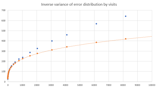 |
| Blue dots are the empirical precisions, orange is a power-law fit to the points less than 1000 visits. |
 |
| The same plot, showing only the points for less than 1000 visits, on a log-log scale. |
It seems like the variance decreases very rapidly at the start, more than one might expect treating the visits as i.i.d observations of a noisy value (in such a case, the precision should increase linearly, here the first few visits reduce the error variance or increase the precision much more than the later ones). It does appear to become linear for larger numbers of visits, but initially scales more like a power law.
Inspired by these observations, I implemented a simple model where rather than equal-weighting all playouts within a subtree and averaging their values to produce the parent value, the playouts of each child were instead weighted by a very rough approximation of the likelihood that the given child had the best value, modelling the error distribution of a child as a t-distribution with 3 degrees of freedom with precision that scaled as a function of the number of visits in that child (using a much simpler and more conservative scaling than the one observed). And so on, recursively through the whole search.
For example, this causes a new child with with a good value that has received enough visits to make it likely to be better, even taking into account the heavy tail distribution of errors, than an old child with many more visits, to be significantly upweighted relative to the old child. This causes the parent node's value to react more quickly to thew new child's value. Reversewise, if a few visits are put into a child and get extremely bad results (perhaps due to the NN policy being mistaken about a particular tactic), that child will be downweighted, causing those visits to influence the parent slightly less than equal-weighting would. In this manner, the MCTS becomes slightly more minimax-like and quicker to react to new refutations.
I tried integrating various powers of the weighting factor into the actual MCTS search, to see the effect of applying different amounts of this weighting on the strength of the bot:
Elo ratings by bot, 800 visits:
v49-140-800v-m50%-fp16: 548.9  75cf ( 545.9, 551.9)  95cf ( 543.9, 553.9)  (16389.0 win, 15191.0 loss)
v49-140-800v-m70%-fp16: 544.4  75cf ( 540.4, 548.4)  95cf ( 538.4, 550.4)  (7793.0 win, 7704.0 loss)
v49-140-800v-m30%-fp16: 541.9  75cf ( 537.9, 545.9)  95cf ( 535.9, 547.9)  (7725.0 win, 7771.0 loss)
v49-140-800v-m00%-fp16: 535.6  75cf ( 531.6, 539.6)  95cf ( 529.6, 541.6)  (9733.0 win, 10294.0 loss)

m00% = no model
m30% = use pow(model,0.3) as final weighting
m50% = use pow(model,0.5) as final weighting
m70% = use pow(model,0.7) as final weighting
It took quite a large number of games over many days to establish statistical significance, but it seems like applying part of this weighting does give a small strength increase! Or at least, it does for this particular neural net and for the current values all the other search parameters involved (cPUCT, FPU, etc), and only a small increase. Which I found still pretty cool. I haven't had the chance to do further experimentation in this area since this test, but it's definitely an area that I think would be worth revisiting in the future.
